In the previous lecture, we covered the basics of how CCDs work. Once we have taken our CCD image we'd like to use it for some scientific purpose. For example, we might wish to perform relative or absolute photometry on the stars in the image. However, before we can do that, we must perform some additional processing on the image. To understand why, we need to look at some details of CCD operation.

Bias Frames

Let's recall how a CCD measures the number of electrons \(N_e\) in each pixel. These electrons have a total charge \(Q = eN_e\). We measure this charge by dumping it onto a capacitor with capacitance \(C\) and measuring the voltage \(V = Q/C\). We can re-write the number of electrons in terms of this tiny, analog voltage as \[N_e = CV/e.\] In other words, the voltage is proportional to the number of electrons. Because we need to store the data in digital format, the analog voltage is converted to a digital number of counts \(N_c\), by an analog-to-digital converter (ADC). Since the value in counts is proportional to the voltage \(N_c \propto V\), it follows that the number of counts is proportional to the number of photo-electrons, i.e \(N_e = GN_c\), where \(G\) is the Gain, measured in e-/ADU. The number of bits used by the ADC to store the count values limits the number of different count values that can be represented. For a 16-bit ADC, we can represent count values from 0 to 65,535.

Now, imagine a relatively short exposure, taken from a dark astronomical site. Suppose that the gain, \(G=1\) e-/ADU and that in our short exposure we create, on average, two photo-electrons from the sky in each pixel. Because of readout noise, we will NOT have 2 counts in each pixel. Instead, the pixel values will follow a Gaussian distribution, with a mean of 2 counts, and a standard deviation given by the readout noise, which may be of the order of 3 counts. It should be obvious that this implies that many pixels should contain negative count values. However, our ADC cannot represent numbers less than 0! This means our data has been corrupted by the digitisation process. If we didn't fix this, it would cause all sorts of problems: in this case it would lead us to over-estimate the sky level.

The solution is to apply a bias voltage. This is a constant offset voltage applied to the capacitor before analog-to-digital conversion. The result is that, even if the pixel contains no photo-electrons, the ADC returns a value of a few hundred counts, nicely solving the issue of negative counts. However, it does mean that we must correct for the bias level when doing photometry! Each pixel in our image contains counts from stars, from the sky background and from the bias level. We must subtract the bias level before performing photometry.

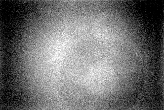
How do we know what the bias level is? The easiest way to do this is to take a series of images with zero exposure time. Because there is no exposure time, these images contain no photo-electrons, and no thermally excited electrons. These images, known as bias frames, allow us to measure the bias level, and subtract it from our science data. A bias frame is shown in figure 73. Several bias frames are needed because the value of any pixel in a given bias frame will differ from the bias level due to readout noise. Averaging several frames together reduces the impact of readout noise and gives a more accurate estimate of the bias level. The master bias frame produced from this averaging can be subtracted from all science images to remove the bias level from each pixel.

---

Dark Frames

Recall that photo-electrons are produced in CCDs by photons exciting electrons from the valence band to the conduction band. However, this is not the only way to excite electrons into the conduction band. Thermal excitation is also capable of producing electrons in the conduction band. Thermal excitation of electrons is known as dark current and the electrons produced by it are indistinguishable from photo-electrons.

Dark current can be very substantial. At room temperature, the dark current of a standard CCD is typically 100,000 e-/pixel/s, which is sufficient to saturate most CCDs in only a few seconds! The solution is to cool the CCD. The typical operating temperatures of CCDs are in the range 150 to 263 K (i.e. -123 to -10℃). At major observatories, most CCDs are cooled to the bottom end of this range, generally using liquid nitrogen. The resulting dark current can be as low as a few electrons per pixel per hour. The CCDs on the Hicks telescopes are air-cooled to a few degrees below zero, and have dark currents of around 40 e-/pixel/hour.

Neither of these values are negligible, especially for short exposures. Thus, every pixel in our image contains contributions from stars, sky background, bias level and dark current. The dark current must be measured, and subtracted from our science images for the same reasons as the bias level. For this purpose dark frames are taken. These are long exposures, taken with the shutter closed. These frames will have no contribution from photo-electrons, but they will contain dark current and the bias level. This means that dark frames must have the bias subtracted from them before use. Once the bias level has been subtracted off, several dark frames can be combined to make a master dark frame, which can be subtracted from your images.

It is best to combine the dark frames using the median, rather than the mean. Dark frames are often long exposures, which can be affected by cosmic rays. Cosmic rays hitting the CCD will excite also excite electrons. Taking the median of the master dark will help remove cosmic rays from the master dark frame.

Because the dark frame increases with time, it is easiest if the dark frames have the same exposure time as your science images. If they do not, it is possible to scale the dark frame by the ratio of exposure times, since dark current increases (roughly) linearly with time. Dark current is also a strong function of temperature - it is essential that dark frames are taken with the CCD at the same temperature as your science frame.

Figure 74 shows an example dark frame. In this 300-sec exposure the dark current is about 50 counts. Note that not every pixel has the same value. Some of this is read noise, but it is also true that different pixels in a CCD show different levels of dark current. Some pixels show very high levels of dark current - these so called hot pixels can have a very serious effect on your photometry if your target star happens to lie on top of one.

---

Flat Fields

Suppose we use our telescope and CCD to take an image of a perfectly uniform light source. Would every pixel have the same number of counts in it? No - as we have seen each pixel will have a varying contribution from dark current and readout noise. What if we ignored these effects? The answer is still no. Various effects combine to mean that the count level can vary significantly across the image. Figure 75 shows an image of the twilight sky taken with the ROSA telescope on the roof of the Hicks building. On the small image scale of a telescope, the twilight sky is an excellent approximation to a uniformly illuminated light source. However, figure 75 is far from uniform.

There are three main reasons for the structure seen in figure 75.

Vignetting

Consider the design of the Newtonian telescope shown in figure 41. If the secondary mirror is exactly the right size to fit the beam produced by an on-axis source, some fraction of the beam produced by an off-axis source will miss the secondary mirror. This light will be lost, and off-axis sources will appear dimmer than on-axis sources. This is vignetting, and its effect is clearly visible in figure 75.

Pixel-to-Pixel variations

Each pixel in a CCD is not exactly the same size; manufacturing tolerances mean that some pixels are larger than others. If each CCD pixel is exposed to a constant flux, the variation in pixel area means that some pixels will capture more photons than others. This effect can also be seen in figure 75 if you look closely, and is often called flat field grain.

Dust grains on optical surfaces

Dust grains on the window of the CCD, or on the filters will block out a small fraction of the light falling on the CCD. These grains appear as dark donuts, with the size of the donut depending on how far from the focal plane the dust grain is. Two such donuts are visible in figure 75.

Flat field frames

It is essential to correct our images for these effects. If we did not, the number of counts from an object would vary depending upon its location in the image, ruining our photometry. Fortunately, we can correct these effects using flat field frames. These are images taken of the twilight sky, which is assumed to be uniform (this is a good assumption for most instruments). Any variation in the flat field is therefore due to the effects above. Because vignetting and the contribution from dust grains can depend on the filter, flat fields must be taken in the same filters as your science data.

For small telescopes, it can be more convenient to use a specially constructed flat-field panel, such as the one shown in figure 76. These panels are carefully designed to provide a uniform light source. The advantage of a flat field panel over the twilight sky is that flat fields can be taken at any time, whereas twilight flats can only be taken in a narrow window after sunset.

How should the flat field be used? First of all, we must realise that the flat field image must be bias subtracted. Dark frame subtraction is not normally necessary, since exposure times are short and the dark current will be very small. The count level of pixel \((i,j)\) in the bias-subtracted flat field image can be written as \[F_{ij} = \alpha_{ij} F,\] where F is the uniform flux of the twilight sky, or flat field panel. The quantity \(\alpha_{ij}\) represents the fraction of light lost to vignetting, pixel-to-pixel variations and dust grains. If we normalise our image, i.e. divide the flat field by the mean flux, \(F\), we get an image whose brightness \(f\) is given by \(f_{ij} = \alpha_{ij}\). Our science image is given by the product of the flux falling on each pixel \(G_{ij}\), and the flat field effects, giving an image in which the brightness of pixel (i,j) is given by \[G'_{ij} = G_{ij}\alpha_{ij}.\] Dividing our science image, \(G'_{ij}\) by the normalised flat field image, \(\alpha_{ij}\), gives the actual flux falling on each pixel \(G_{ij}\), as desired.

---

A worked example - M52

The calibration frames shown in the figures above were taken to support observations with ROSA of the nearby galaxy M52, by a first year student in 2012. A raw CCD image in the I-band is shown in figure 77. Five sets of each calibration frame were taken. The five biasses were median-combined to make a master bias. The darks were bias-subtracted and median-combined to make a master dark. The flat field images were bias subtracted and median-combined to make a master flat, which was normalised. The raw CCD image then had the master dark and bias frames subtracted, and was divided by the normalised master flat to make the calibrated CCD image, also shown in figure 77.

Note that the calibrated image has had the dark current from hot pixels removed. If you look closely, you can also see that the illumination across the frame is even (as vignetting has been corrected), and that the pixel-to-pixel variations have been removed.

Many science images in the BVI filters were taken, and calibrated as above. These were then aligned to correct for imperfections in telescope tracking, and combined into the colour image seen in figure 78.