In this practical you will learn to do relative photometry on astronomical data. Our example dataset will
be data on the delta-Scuti star SZ Lyn. The data was taken by third-year students using
the department's remote controlled 10-inch telescope, ROSA.
We know how to do aperture photometry in principle. In practice, there
are many software packages available to perform aperture photometry. We will analyse our images using
AstroImageJ. This software package
is freely available, runs on Windows, Linux and OS X and does not have a steep learning curve.
There is a Python library designed for
performing photometry on images. However, it’s use can be quite complex, so we’ll focus on using easier
tools!
The Data
You will need a copy of the data. The data files can be found using Windows Explorer at
ThisPC/shared/Student/PHY_Share/Public/PHY241/SZLyn. There are 427 images of SZ Lyn, taken
over several hours. Each image is stored in a file format called FITS format, and end in the .fit
extension. FITS format is the standard image format for astronomical data. Inside one file is both the
image, and a header, which contains metadata about the image - such as when it was
taken, and what filter the data was taken in.
Do not copy the SZ Lyn FITS files to your shared folders (U: drive). The data is nearly
half a gigabyte, and will fill your allocation of networked drive space!
Instead, copy the SZ Lyn folder to C:/MyFolder/phxxxx, where "phyxxx" is your University username. This
copies the files to the hard drive of the machine you are sitting in front of, for rapid access.
You MUST delete anything you place in this directory at the end of the session.
The Software
Instructions for installing AstroImageJ are below. Should you ever want to download a copy for your own
machine, it is available for download here. A detailed and helpful manual
is available here.
If you encounter difficulty, or do not understand a setting, check the manual.
Task 0: Install AstroImageJ. Using Windows Explorer, copy the ZIP file
fromAstroImageJ\AstroImageJ.exe
ThisPC/shared/Student/PHY_Share/Public , and save it on your computer. Locate the file in
Windows Explorer, right-click and choose "Extract All". This will create a folder
starting with AstroImageJ. Inside that folder is another folder called AstroImageJ.
You can run the program by double-clicking on AstroImageJ\AstroImageJ.exe.
Note: You may get several windows asking for permission to run the program. Click
"OK" to these. If you get a window requesting permission for AstroImageJ to get through a
FireWall, click cancel on that window only.
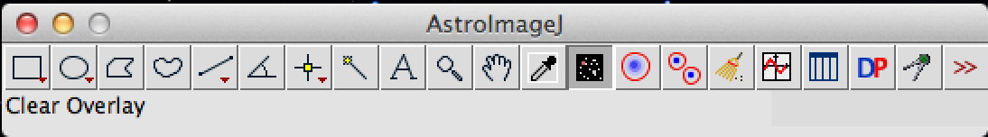
Task 1: Open AstroImageJ. You are presented with the main window, as seen in figure 14.
Load all of our images by choosing File > Import > Image Sequence... Navigate to the
folder that contains all the .fit images, select one, and click Open.
You will be presented with a second window presenting options for loading an image sequence. Here it
is extremely important that you tick the Use Virtual Stack box. If you
don't the PC will attempt to store every picture at once into it's memory. You may get lucky, or you
may cause your PC to grind to a painful halt.
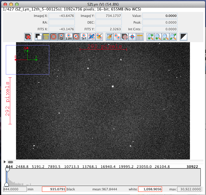
You should see a new window open, with a display of the first image in the stack. This is the
photometry window, shown in figure 15. Near the bottom of the photometry window
is a slider which moves through the images, and a button, which will animate
through all the images in the stack. Press this button and notice how the stars move around slightly
with time. This is due to imperfect tracking of the telescope. Note also the subtle changes in size of
the stars as the seeing changes from frame to frame, and the random
occurrence of bright pixels as they are struck by cosmic rays.
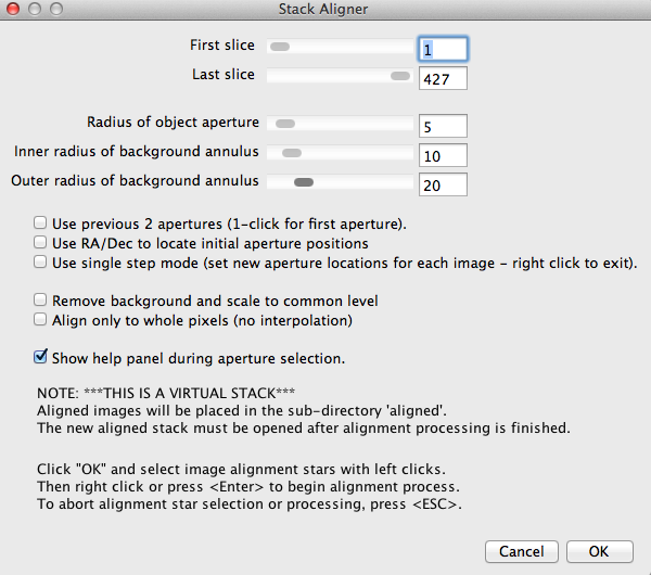
Task 2: Align the images by choosing Process > Align stack using WCS or
apertures... This brings up the stack aligner window (figure 3). Make sure the Use
previous N apertures box and the Align only to whole pixels boxes are
unchecked. Make sure the Show help panel box is checked.
The radii of the object aperture and sky annuli are not too important, but you might want to make
sure the object radius is set to a reasonable value, since if the star lies outside this radius,
AstroImageJ will not be able to calculate the image shift. Set this value to somewhere in the range
15-20.
Click OK to begin selecting stars to use for alignment. Left click on a star to add an
aperture around it. Add two or three bright stars to use for alignment and press Enter or
right-click to begin the alignment procedure.
AstroImageJ will now look for a star within each aperture, and measure the centroid of those stars.
For each image, it uses the centroid of the stars to estimate the image shift.
When AstroImageJ has finished, you should have a new ImageSequence already loaded called "Aligned".
Hit the button to run through the images and check the alignment.
Now it is time to perform the relative photometry on the aligned images. Recall that aperture photometry
involves three steps, centroiding, sky background estimation and extraction of the counts from our
object. AstroImageJ performs all three of these steps with the Multi-Aperture Photometry tool. First
however, we need to know how large to make our object apertures, and the inner and outer radius of our
sky annulus. To do that we need to know what the FWHM of the stars in our image is.
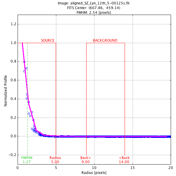
Task 3: In the photometry window, click on a star, then choose Analyze > Plot Seeing
Profile... You should end up with a plot like figure 17. Based upon
this plot, decide how large you want your aperture sizes to be.
You will need to consider what effect using an aperture that is too small, or one that is too large,
may have on your data.
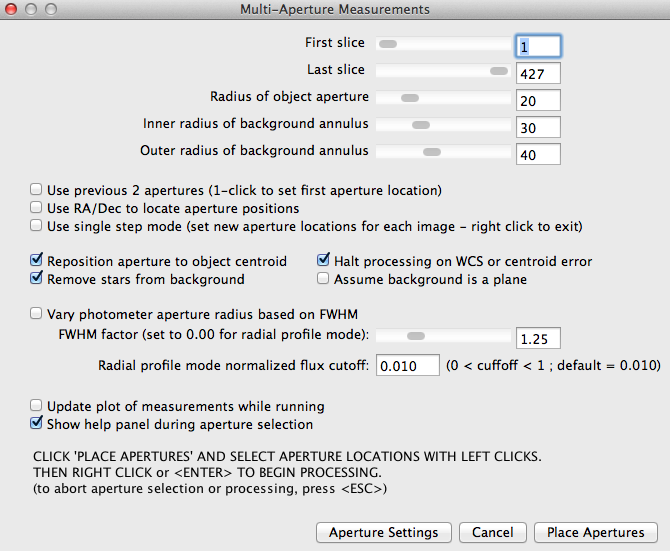
Task 4: Open the Multi-Aperture photometry tool by choosing Analyze >
Multi-aperture... Set the radius of the object aperture, and the inner and outer radii of
the background annulus to the values chosen earlier.
Make sure the various options boxes are marked as indicated in figure 18, and click
Place Apertures to begin. Aperture placement is done in exactly the same way as when you
aligned the images.
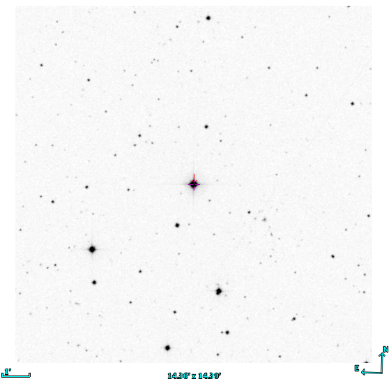
Figure 19 shows a plot of the sky centred on SZ Lyn. The orientation of this image is
not the same as the images from ROSA. Place your first aperture around SZ Lyn, and at least one
other aperture around a comparison star. When choosing a comparison star, you should choose an
unsaturated, bright star. If possible, it should be brighter than SZ Lyn. Why?
Once you've placed your apertures, right-click or press Enter to start performing
photometry.
Task 5: Save your data to a Tab-Separated Values text file by clicking in the Measurements
window and choosing File > Save As...
You have two options to make a plot from the data in this file. You can use Excel, or upload the
saved file to CoCalc and plot it using Python. If you choose the latter route, you will find the
text file hard to read in using NumPy, because some of the columns don't contain numbers. Instead,
you can use the Pandas library instead, and use something
like the following code snippet to read in the file:
# use the Pandas library
import pandas as pd

# read in the data, explaining that columns
# are separated by tabs (\t)
data = pd.read_csv(delimiter='\t')

# you can access data directly by column name
x = data['J.D - 2400000']
y = data['rel_flux_T1']
Use your preferred method to make two scatter plots, one of JD vs
Source-Sky_T1 and another of JD vs rel_flux_T1.
Notice how using relative photometry has corrected the large jump that occurs in the plot of the
counts from the target star. This jump is associated with a change in position of the stars, but it
has affected our target and comparison star equally, so it is not present in the count ratio plot.
Now you have successfully learnt to use AstroImageJ for aperture photometry. However there are two issues
remaining. The first is that your lightcurve does not have accurate error bars. The second is that you
do not know if you used the best aperture sizes. Before we can calculate error bars we need to know more
about how CCDs work. We will cover that later in the course.
However, we can fix the second problem.
Task 6: Re-run your aperture photometry with a few different aperture sizes, and
save the results. You will need to Clear the Measurements table each time. Leave the sky
annulus unchanged for now, and simply change the object aperture radius.
For your new measurements plot JD vs rel_flux_T1 in each case. Try
to plot them on the same graph, and add a small offset to each dataset in y, so you can see the
curves.
Which aperture size is best? What does the light curve look like when the object aperture is too
small? What happens when it is too big? See if you can understand these effects.
One final thing to think about - if you use a small aperture radius like 2 pixels, much of the light
from your object is falling outside your aperture. Why do you still get a reasonable lightcurve?