P05: Absolute Photometry using VO software


In the previous lecture, we learnt the theory behind precise calibration of photometry, enabling us to put photometric observations onto a standard scale with precisions of better than 1%. In this practical we are going to learn how to produce calibrated photometry using a simplified method. This method does not yield the same accuracy as an analysis using observations of primary or secondary standard stars, combined with the use of colour terms. On the other hand, it is much simpler to apply, and even works to produce calibrated photometry through thin cloud. If you are happy to accept accuracies on the order of a few percent, I recommend using the method described below whenever you need to produce calibrated photometry.

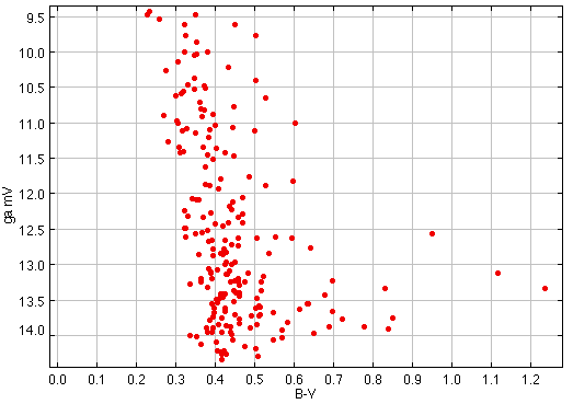
In this practical, we will produce a colour-magnitude diagram of the young open cluster NGC 869, using readily available software. First, I describe the method which will enable us to obtain calibrated magnitudes.

Method

In the last lecture we saw that, for any star, the difference between the calibrated magnitude, \(m\) and the above-atmosphere instrumental magnitude \(m_{0,i}\) is given by: \[m = m_{0,i} + m_{\rm zp},\] where \(m_{\rm zp}\) is known as the zero point. The above-atmosphere instrumental magnitude is given by: \[m_{0,i} = m_i - kX,\] where \(m_i = -2.5 \log_{10} \left( N_t/t_{\rm exp} \right)\) is the instrumental magnitude, \(k\) is the extinction coefficient, and \(X\) is the airmass. Therefore: \[m = m_i - kX + m_{\rm zp}.\] In other words, if we were to plot the calibrated magnitude \(m\) against instrumental magnitude \(m_i\) for all the stars in our image, we would expect a straight line, with a gradient of one, and an intercept equal to \( kX + m_{\rm zp} \). This intercept could then be added to all of our instrumental magnitudes to produce calibrated magnitudes.

What makes this technique possible, is the existence of large sky surveys, which have provided calibrated magnitudes for many, relatively bright stars over a very wide areas of the sky. If your data is covered by one of these surveys, and it provides calibrated magnitudes in the same filter as your data, you can apply this technique relatively quickly.

Accuracy

The accuracy this technique can achieve is limited by two factors. First of all we are not taking into account any secondary effects, such as 2nd-order extinction, or colour terms. Secondly, our photometry cannot be any more accurate than that in the sky survey we use. Typically, large sky surveys achieve accuracies of a few percent. Ignoring the secondary effects will probably introduce errors on a similar level. If you need calibrated photometry to better than a few percent, you will have to observe standard stars, and apply the rigorous method described in the previous lecture.

Steps

Applying this method requires the application of four steps. These steps are:

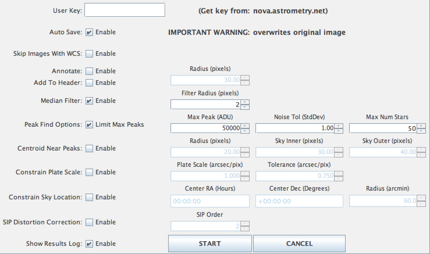
  1. astrometric solution of the image - so we know the RA and Dec of all the stars we measure in our image;
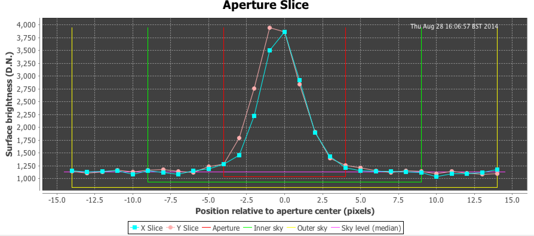
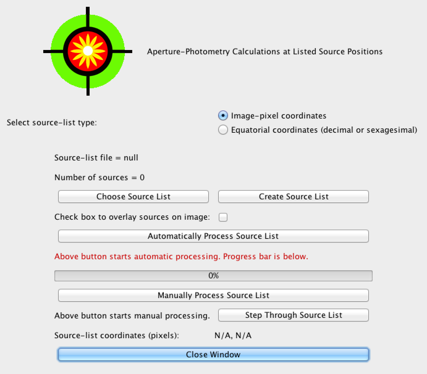
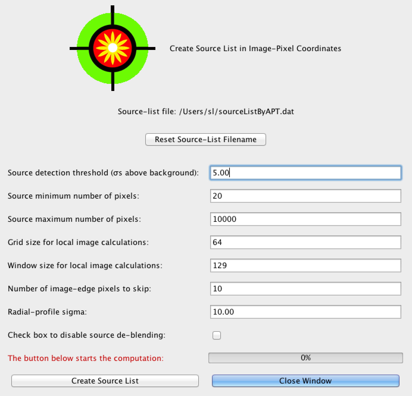
  2. finding the stars in our image, and calculating instrumental magnitudes;
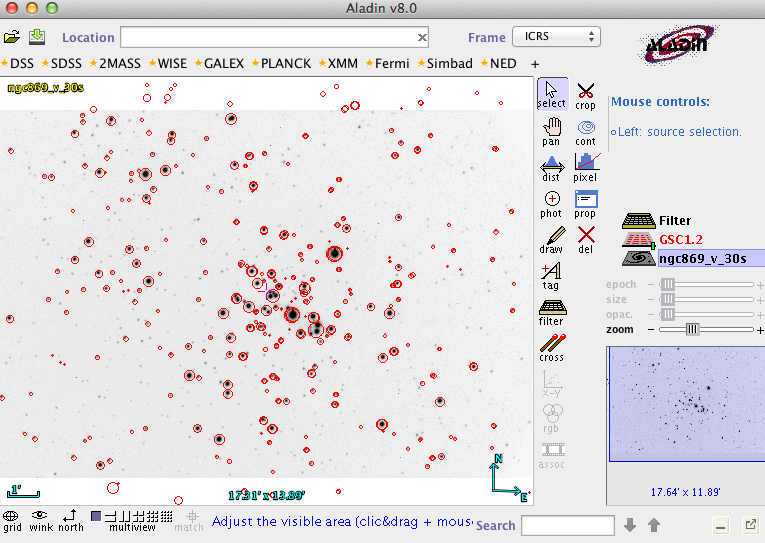
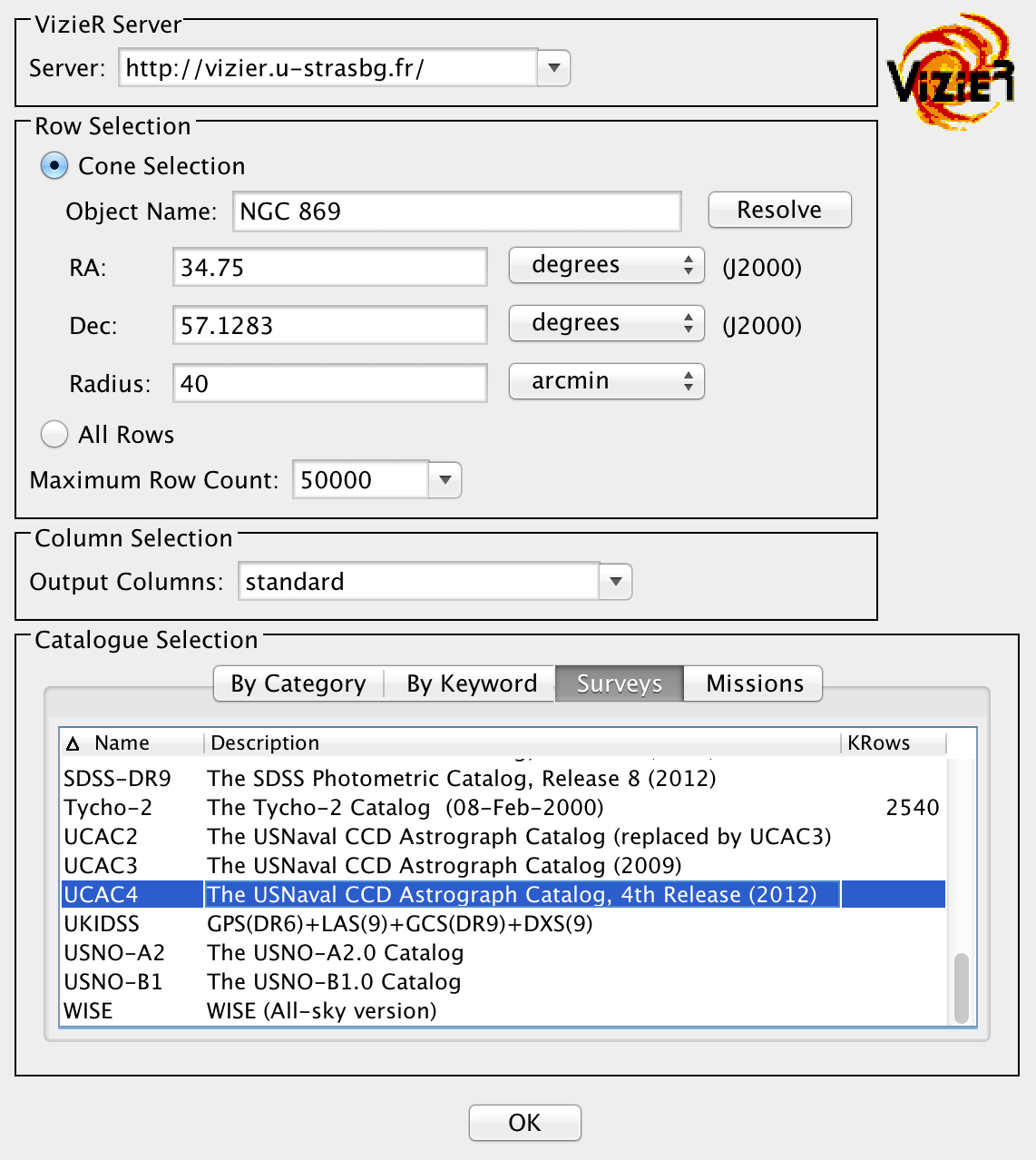
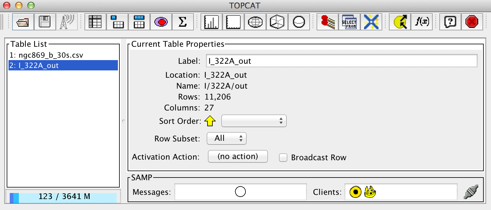
  3. matching our stars against a sky-survey, so we know instrumental and calibrated magnitude for many stars;
  4. calculating the offset between instrumental and calibrated magnitudes, and applying to all stars in our image.

We will need to use several software packages to perform these steps and achieve our goal. Following the guide below will show you how to achieve this with readily available, cross-platform software packages.

The Data

You will need a copy of the data. The data files are located at C:\SharedFolder\astrolab\NGC869\Images.

You don't need to copy the data from this location to work on it, but this folder is local to the PC you are working on now. If you want to save these files for later, you will need to copy them to your M: or U: drives.


Astrometric Calibration

Eventually we are going to match our instrumental magnitudes for each star, against calibrated magnitudes from a catalog which comprises of RA, Dec and magnitude. Thus we will need to know the RA and Dec of every star we calculate an instrumental magnitude. We do this by ensuring the image file has an astrometric solution - a piece of metadata which allows software to convert between pixel positions (x, y) and sky coordinates (RA, Dec).

For the data in today's practical, this step has already been carried out, and the image has an astrometric solution already. This section is included for reference if you use these notes to reduce your open cluster data. If you are just working through the practical, skip ahead to the section on aperture photometry.

You can create an astrometric solution for your images using AstroImageJ, which we encountered in the previous practical. AstroImageJ has a tool to automatically find the RA and Dec of an astronomical image, using an online web tool called Astrometry.net. To use this service, you will need to sign up for an account at http://nova.astrometry.net. Once you have logged in, go to "Profile" and make a note of the API key listed there - you will need it to use astrometry.net from within AstroImageJ.

Task 1: Open AstroImageJ. Load the B-band image by choosing File > Open. The astrometry solution can be controlled by choosing WCS > Plate Solve Using Astronometry.net (with options). A window like the one shown in figure 26 will appear.

There are lots of options. The options for Median Filter and Peak Find Options control how stars are detected in the image. You probably want to uncheck these to start with, but if your images are very noisy, Median Filter can prevent the spurious identification of noise as stars. Peak Find Options can be used to prevent the use of saturated stars, whose positions are unreliable.

The option SIP Distortion Correction will enable a more complex transformation between pixel position and RA, Dec which can correct for aberrations introduced by the telescope optics. You should usually check this box.

Astrometry.net can usually find a solution for many images without an initial guess of the RA and Dec of the image. Try this by entering your astrometry.net API Key into the User Key box and clicking Start. Check the output log to see if the astrometric solution was successful.

If it wasn't, you may need to give Astrometry.net some constraints on the image location. To do so we need to know the rough position the telescope was pointed at and the image scale (in arc seconds per pixel). In our case, the RA was roughly 02:18:57 and the Dec was roughly +57 08 46. The image was taken with 2x2 binning, and so the pixel scale is 1 arc second per pixel (image scales for the Hicks Observatory can be found here). You can make Astrometry.net search only around these values by ticking the Constrain Plate Scale and the Constrain Sky Location checkboxes, and entering appropriate values in the relevant text boxes.

Figure 26: The astrometry window in AstroImageJ. You must put your astrometry.net API key in the User Key box. If the Auto Save checkbox is ticked, your image will automatically be overwritten by one with an astrometric solution.

Once we have a successful astrometric solution, we can move onto the aperture photometry. In figure 27 I show the B-band image of NGC 869 displayed using the software Aladin. Also shown is data from an all-sky catalog. The fact that the catalog objects line up with the stars in the image show that the astrometric solution is accurate.

Figure 27: A well-calibrated image of NGC 869. Notice how the stars and catalog objects line up. This tells us the conversion between pixel coordinates and sky coordinates is accurate.


Aperture Photometry

We have done aperture photometry before, using AstroImageJ. Whilst this tool is excellent for relative photometry, and producing light curves, each aperture must be placed by hand, which makes it onerous to use when we want to measure every star in an image. For this reason I will introduce a new software tool, the Aperture Photometry Tool, or APT for short.

APT can be installed on Windows, Linux or Mac machines. There is excellent documentation, and a 35-minute long video tutorial. Should you need to perform aperture photometry on a large number of stars in your course, it is a good place to start.

APT is installed on the astrolab machines under C:\SharedFolder\astrolab\APT_v2.4.7. Double click on the Application in this folder to run APT.

Task 2: Setup APT.

Start APT and click Open Image to load your astrometrically calibrated image. Click on More Settings and make sure the source algorithm is set to model 0 (this is straightforward aperture photometry), and the sky algorithm is set to model B (this will use a sky annulus to measure and subtract the sky background). Click Apply Settings and then Close Window.

Now we need to set our aperture settings, but we'll need to find the FWHM so we know roughly what settings to use. Click on an isolated star in the image to place an aperture around it. Then click on Aperture Slice. You will see a plot with two cross sections across your star, one horizontal, one vertical (see, for example, figure 28). You can use this plot to estimate the FWHM of stars in your image.

Once you know the FWHM, use it to set the values for your photometry apertures. You should have some experience in this from the relative photometry practicals, but decent starting values are an object aperture radius of 1.5xFWHM, an inner sky radius of 2xFWHM and an outer sky radius of 3xFWHM.

Click on the big button in the GUI (labelled something like 5/5/0 -> Alter) to set the aperture parameters. Two windows should appear. The Major radius in the larger window is where you enter the object aperture. Click Apply. The sky annulus radii are entered in the smaller window. Set these values and click Apply. Close both windows.

Figure 28: An aperture slice plot from APT, showing horizontal and vertical slices across the image. In this example, the peak of the star is around 2500 counts above the background, and the FWHM is roughly 3 pixels. Using these numbers, reasonable values for the aperture sizes have been set, and are shown on the plot.

Source Detection

With your apertures set, you can perform aperture photometry on any single star by clicking on it. Have a go at this, and look at the values reported in the Aperture Photometry Results area of the APT window. However, we want to detect all the stars in the image, and perform aperture photometry on all of them at once.

Task 3: Click on the Source List button at the bottom of the APT screen. The source list tool will appear (figure 29). Click Create Source List to get the source list creation tool, also shown in figure 29. Make sure the settings are as in figure 29. The important settings are the detection threshold, which sets how bright an object must be to be detected, and the Radial-profile sigma which gives APT an idea how large the stars in the image will be. This last value wants to be at least twice the FWHM.

When the settings are correct, click Create Source List, and close the window once processing is complete. You can view the detected sources by ticking the "Check box to overlay sources on image" checkbox in the source list tool.

If you're not happy with the detected sources, you can tweak the parameters and try again.

Photometry

Now we have a list of detected sources, and we have set our apertures, we can go ahead and perform aperture photometry on all the sources.

Task 4: In the source list tool, click Automatically Process Source List, to perform aperture photometry with the current aperture settings on all stars in the source list. Close the source list tool window when complete.

You can view your results by clicking List Results at the bottom of the APT window. Click on Export Contents to save your results to a text file that can be used by other programs. In the window that appears click Reset CSV Filename to set the filename to something useful (in this practical, use NGC869_B.csv) and click Create CSV File. You might want to save this file to your U: drive, so it is available later.

It is important to note that the results file is not cleared each time you load a new image, or restart APT. Unless you clear it manually, the old results will still be present. Before you close the results window, click Clear Contents to empty the current results.

Figure 29: Left: Top: The APT source list window Right: Bottom: The APT create source list window, with reasonable settings for the images in this practical.

Photometric Calibration

Now you should have a CSV file, called NGC869_B.csv, with your instrumental magnitudes (and much besides) in it. The next step is photometric calibration. As a reminder, this involves fitting a straight line to a graph of instrumental magnitude against calibrated magnitude, to find the offset between the two.

This can be done inside APT itself, but slightly annoyingly APT requires files in a new format. The file format is space-separated, with three columns: RA, Dec and Magnitude. To get our instrumental magnitude data into this format, and to download calibrated magnitudes covering our image, we will introduce a new tool - Topcat.

Topcat is an amazing tool for manipulating tables of astronomical data, and for accessing the wealth of data available over the web. Like all the software used in this practical it is cross-platform and freely available. It's rich functionality is described in detailed documentation. Topcat is installed on the astrolab machines under C:\SharedFolder\astrolab\topcat.

Task 5: Start Topcat and load your instrumental magnitude file by choosing File > Load Table. The load table dialog is used to load data from a wide range of sources, including web-based catalog data, so it is slightly complex. You will need to set the Format drop-down box to CSV and navigate to your file (NGC869_B.csv) using the System Browser.

Now we will save our data to a simple text format, but we only want three columns - RA, Dec and Magnitude. To control which columns are shown in Topcat, and which columns are exported choose Views > Column Info. Make sure the only columns ticked are ApertureRA, ApertureDec and Magnitude. Close the column info window.

Now export our data by choosing File > Save Table(s)/Session. Set the output format to ascii and choose a save location using the System Browser. Name your file NGC869_B_instrumental_mags.txt.

Now we have one of the two files required. We need to get catalog data for this part of the sky, and in the correct filter. The UCAC4 catalog is a catalog which combines other sky surveys to provide data in many filters across much of the sky. Crucially, in this case it includes B and V magnitudes, the two filters used for NGC 869. We can download the part of the UCAC4 catalog we need, and export to the correct format, using Topcat.

Task 7: Inside Topcat, choose VO > VizieR Catalogue Service. In the window that opens, make sure the Cone Selection checkbox is selected. Enter NGC 869 in the Object Name, and click Resolve. Topcat will fill in the RA and Dec for NGC 869 for you. Next we set the area of catalog we want to download. Our image is about 20 arc minutes on it's long edge, so set the Radius box to 40 arcmins.

In the Catalogue Selection part of the window, make sure the Surveys tab is active, select the UCAC4 survey. Check your settings against figure 30 and click OK . Topcat will download the UCAC4 catalogue, and a new table will appear in the main topcat window (figure 31).

We are almost ready to export our UCAC4 data in the same way we did with the instrumental magnitudes. First, however, make sure the UCAC4 table is selected in the main topcat window and choose Views > Table Data. Notice that not every star has a B-band magnitude (the column labelled Bmag). We will need to create a subset of the table, containing only those stars with B-band magnitudes.

Close the table browser. In the main topcat window, choose Views > Row Subsets. In the window that appears, choose Subsets > New Subset. Give your subset a name, and enter "! NULL_Bmag" into the expression box. This will select only those values where the Bmag is not NULL (i.e empty). In the main topcat window, select your subset from the Row Subset drop down box and choose Views > Table Data again. Notice that topcat is now only showing the stars with B-band magnitudes.

Follow the same steps you took in Task 6, to save an ascii file containing only these three columns; RAJ2000, DEJ2000, Bmag. Call this file NGC869_B_calibrated_mags.txt

Figure 30: The VizieR catalog query window in Topcat. The settings shown here will download the UCAC4 catalog data in a 40 arc minute radius around NGC 869

Figure 31: The Topcat main window. Loaded tables are shown in the list on the left. The active table is highlighted. On the right you can change the sort order of the table, and select the active subset.

Now, finally, we have the two files we need to calculate our photometric calibration. This will be done in APT, using the Simple Photometric Calibration tool.

Task 8: In APT, choose Tools > Simple Photometric Calibration. The calibration window will appear (figure 32). Select your saved instrumental magnitude data (NGC869_B_instrumental_mags.txt) by clicking the Choose Uncalibrated Source List button. Do the same for the UCAC4 data (NGC869_B_calibrated_mags.txt) by clicking the Choose Calibrated Source List button.

When we run the tool, it will match the two lists by looking for stars with similar RAs and Decs. We can set the tolerance for this match in the Match Radius box. Set this to 2 arcseconds.

Click the Match Source Lists and Compute Zero Point button. You should get a result something like figure 32. The zero point and uncertainty are shown in the console window (top-right). In this case, the zero point is \(24.24 \pm 0.05\) magnitudes. This is the difference between the calibrated and instrumental magnitudes, and should be added to all of your instrumental magnitudes to give calibrated B-band magnitudes.

The uncertainty in your zero point is important. Changing the zero point will change the location of all of the stars in a colour-magnitude diagram. Therefore, the uncertainty in your zero point should not be combined with the measurement uncertainties in your instrumental magnitude. It will, however, act as a systematic error on the position of stars in your CMD.

We can make our final, calibrated catalog in topcat. Make sure the table containing the instrumental magnitudes is highlighted. Choose Views > Column Info. With the column info window active, choose Columns > New Synthetic Column. Call the column "Bmag" and in the expression box, type "Magnitude + 24.24", where 24.24 should be replaced with the zero point you found in your data.

Use Topcat to save your data in CSV format.


Constructing a Colour-Magnitude Diagram

To make a colour magnitude diagram, we need data in a different filter. I have produced a calibrated V-band catalog from another image, following exactly the steps in this tutorial. The catalog is located at C:\SharedFolder\astrolab\NGC869\Cats.

Task 9: Load the V-band catalog into Topcat, and your own calibrated B-band data. We are going to match them by looking for stars of similar RA and Dec. Choose Joins > Pair Match. Select the Sky algorithm and a Max Error of 2 arc seconds. Select your two tables and choose ApertureRA for the RA Column and ApertureDec for the Dec Column. Click Go.

A new table will be created with the matched stars. This table contains both V and B magnitudes for each star. Following the guidelines in Task 8 for making new columns, make a B-V column, and a column for the error in B-V.

Finally, make a CMD by plotting B-V on the x-axis against V on the y-axis. You can do this either by using the Graphics options in Topcat, or by exporting the new catalog to CSV format and reading it into Excel. You should end up with something like figure 33.

Figure 33: A colour-magnitude diagram for the bright stars in the field of NGC 869, plotted using the 2D plotting option in Topcat.