Calibrating Photometry
Previously, we saw how to extract the sky-subtracted signal from
an object, measured in counts, from an image. Once this has been done, it is useful to convert
to a magnitude in a photometric system. To see why this is important imagine two astronomers
observing the same star, through the same filter, but with very different telescopes. Clearly an
astronomer with a large telescope is going to measure more counts than the unfortunate
astronomer who has a small telescope. It is therefore not very meaningful to share our results
with others in units of counts.
Converting a measurement in counts into a calibrated magnitude involves five steps:
- divide the number of counts by the exposure time, to get a measure of flux in counts per
second;
- calculate the instrumental magnitude, from the counts per second;
- determine the extinction coefficient, and correct the instrumental
magnitude to the above-atmosphere value;
- repeat the above steps for a standard star and use the resulting above-atmosphere
instrumental magnitude of the standard star to calculate the zero point;
- use the zero point to transform the above-atmosphere instrumental magnitude of the target
star to the required photometric system.
The above steps are described in more detail below.
Instrumental Magnitudes
Let us call the sky-subtracted signal from our target object, in counts, \(N_t\). We convert this
to an instrumental magnitude, using the formula
\[ m_{\rm inst} = -2.5 \log_{10} \left( N_t / t_{\exp} \right), \]
where \(t_{\rm exp}\) is the exposure time of the image in seconds. The instrumental magnitude
depends on the characteristics of the telescope, instrument, filter and detector used to obtain
the data. It is therefore meaningless to compare two instrumental magnitudes taken under
different situations, without first putting them on a calibrated scale.
The relationship between instrumental magnitudes and calibrated magnitudes can be understood as
follows. The counts per second \(N_t / t_{\exp}\) is proportional to the flux, \(F_\lambda\).
Hence
\[ m_{\rm inst} = -2.5 \log_{10} \left( \kappa F_\lambda \right) = -2.5 \log_{10} F_\lambda +
c',\]
therefore, instrumental magnitudes are offset from calibrated magnitudes by a constant:
\[ m_{\rm calib}= m_{\rm inst} + m_{\rm zp},\]
where the constant, \(m_{\rm zp}\), is known as the zero point. The zero point
depends upon the telescope and filter used. We can understand this because if we used a larger
telescope to observe a star, the instrumental magnitude would change, but the calibrated
magnitude must not!
A handy tip to remember about zero-points is this; an object with a calibrated magnitude equal to
the zero point gives one count-per-second at the telescope. For example, suppose the zeropoint
of a telescope/filter combination is \(m_{\rm zp} = 19.0\). If we observe a star with \(m_{\rm
calib}= 19.0\), then it follows that, for this star \(m_{\rm inst}=0\). By definition then, this
star gives one count-per-second.
Extinction
The next step is to convert the instrumental magnitude, which is measured on the surface of the
Earth, to the instrumental magnitude that would be observed above the atmosphere. This is
necessary because the Earth's atmosphere absorbs light from the star, and the amount of light
absorbed depends on the angle of the star above the horizon. If we didn't correct this effect,
observations of objects at different times of night would give different magnitudes! We'll see
how to correct for extinction below, but first we need to work out how
extinction depends on the angle of the star above the horizon.
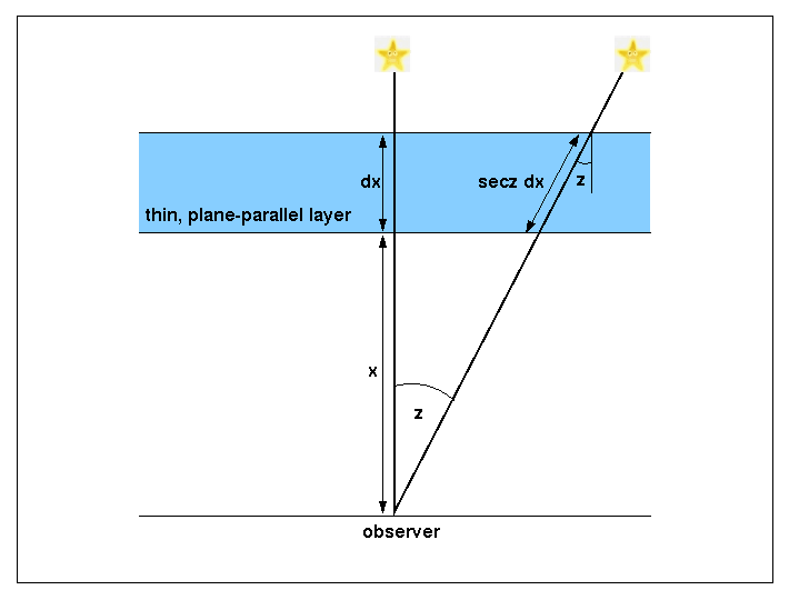
We can derive a simple equation for the extinction correction by assuming the atmosphere is a
series of thin plane-parallel layers. Figure 23 shows such a layer, of
thickness \(dx\) at an altitude \(x\). The path length through the layer for light from a star
at a zenith distance \(z\) is equal to \(dx \,/ \cos z = dx \sec z\). The term \(\sec z\) is
known as the airmass, and is sometimes given the symbol \(X\). At the zenith, \(X= \sec z = 1\),
and this increases to a value of 2 at a zenith distance of 60°. Note that the approximation
of the atmosphere as being plane-parallel breaks down at larger zenith distances. Due to the
amount of extinction, it's a bad idea to observe astronomical objects this low, so we shall not
worry about the curvature of the atmosphere here.
Figure 23: a thin, plane-parallel layer in the Earth's atmosphere. As the zenith distance of the star increases, the path length through the atmosphere increases, and hence the absorption increases. Credit: Vik Dhillon
If the monochromatic flux from an object incident on the layer is \(F_\lambda\) then the flux
absorbed by the layer \(dF_\lambda\) will be proportional to both \(F_\lambda\) and the path
length through the layer. Therefore:
\[ dF_\lambda = - \alpha_\lambda F_\lambda \sec z \, dx,\]
where the constant of proportionality, \(\alpha_\lambda\) is known as the absorption
coefficient, with units of m-1. The absorption coefficient is a function of the composition and
density of the atmosphere, and hence the altitude of the layer, \(x\). We can re-arrange this
equation (and drop the \(\lambda\) subscripts for clarity) to give
\[ \frac{dF}{F} = - \sec z \, \alpha \, dx.\]
Integrating the equation above for \(x\) values from the top of the atmosphere, \(t\), to the
bottom \(b\), we obtain
\[ \int_t^b \frac{dF}{F} = - \sec z \int_t^b \alpha dx.\]
Hence
\[ \frac{F_b}{F_t} = \frac{F}{F_0} = \exp \left( -\sec z \int_t^b \alpha dx \right),\]
where for clarity we have renamed the above-atmosphere flux \(F_t = F_0\) and the flux measured
at the ground by the observer \(F_b = F\). Remembering that the difference between two
magnitudes is \(m_1 - m_2 = -2.5 \log_{10} (F_1/F_2) \), we can write (via some magic with the
change of base formula),
\[m-m_0 = -2.5\log_{10} (F/F_0) = 2.5 \sec z \log_{10}(e) \int_t^b \alpha dx .\]
We define the extinction coefficient, \(k\), as:
\[k = 2.5 \log_{10}(e) \int_t^b \alpha dx,\]
to finally obtain:
\[ m = m_0 + k \sec z = m_0 + kX,\]
where \(m_0\) is the magnitude of a star observed with no extinction (i.e above the atmosphere)
and \(m\) is the magnitude of a star observed at the Earth's surface at zenith distance \(z\).
As an example, if the extinction coefficient from a site in the V-band is \(k=0.15\)
magnitudes/airmass then a star would appear 0.15 magnitudes fainter at the zenith than it would
appear above the atmosphere, and 0.3 magnitudes fainter than above the atmosphere when at a
zenith distance of 60°.
The dominant source of extinction in the atmosphere is Rayleigh scattering by air molecules. This
mechanism is proportional to \(\lambda^{-4}\), which means that extinction is much higher in the
blue than in the red. The extinction can also vary from night to night depending on the
conditions in the atmosphere, e.g. dust blown over from the Sahara can increase the extinction
on La Palma during the summer by up to 1 magnitude. Table 2 lists the
extinction coefficients on a typical (undusty) night on La Palma in UBVRI. For
reference, the night sky brightness on La Palma when the Moon illumination is 0% (Dark), 50%
(Grey) and 100% (Bright) illuminated is also listed. All values in table 2
have been taken from Chris Benn's ING signal program.
| Filter |
\(\lambda_{\rm eff}\) (nm) |
\(k\) (mags/airmass) |
\(m_{\rm sky}\) (mags/arcsec2) |
|
|
|
Dark |
Grey |
Bright |
| U |
360 |
0.55 |
22.0 |
20.0 |
17.7 |
| B |
430 |
0.25 |
22.7 |
20.7 |
18.4 |
| V |
550 |
0.15 |
21.9 |
19.9 |
17.6 |
| R |
650 |
0.09 |
21.0 |
19.7 |
17.5 |
| I |
820 |
0.06 |
20.0 |
18.9 |
16.7 |
Table 2: typical extinction and sky brightness values in the
UBVRI photometric system at a high-quality astronomical site.
Correcting for extinction
To measure the extinction on a particular night, it is necessary to measure the signal from a
non-variable star at a number of different zenith distances. Inspecting the equation \(m = m_0 +
k \sec z\), it can be seen that the extinction would be given by the gradient of a plot of the
instrumental magnitude of the star versus \(\sec z\) and the \(y\)-intercept would give the
above-atmosphere instrumental magnitude. Although such a plot would give the most accurate
answer, it is also possible to obtain an estimate of \(k\) from just two measurements of the
instrumental magnitude of a star at two different zenith distances: subtracting \(m_{z_1} = m_0
+ k \sec z_1\) from \(m_{z_2} = m_0 + k \sec z_2\) eliminates \(m_0\), allowing \(k\) to be
derived.
Note that no explicit extinction correction is required when performing relative photometry. This is because the target and comparison
stars are always observed at the same airmass and hence suffer the same
extinction. Hence, when the target signal is divided by the comparison star signal to correct
for transparency variations, the variation due to extinction present in the comparison star is
removed from the target star.
Aside: Secondary Extinction
For very accurate photometry, the wide bandpass of broad-band filters has to be taken into
account when correcting for extinction. Because extinction is so strongly colour dependent, a
blue object actually loses more light to the atmosphere than a red one. This is true even within
the relatively narrow wavelength range of the UBVRI filters. The solution is to
introduce a colour-dependent secondary extinction coefficient, \(k_2\), which modifies the above
extinction correction equation to:
\[ m = m_0 + k \sec z + k_2 C \sec z,\]
where \(C\) is the colour index, e.g. when correcting a V-band magnitude for extinction, \(C = B
- V\). The secondary extinction coefficient is usually of order a hundredth of a magnitude, so
it will be ignored for the remainder of this course.
Calibrated Magnitude
Now we can find the above-atmosphere instrumental magnitude of any object. The final step is to
observe a primary or secondary photometric standard star to convert to calibrated magnitudes.
Suppose we have measured our instrumental magnitude of the standard star, \(m_{ {\rm std},i }\).
We have also measured the extinction coefficient for the night, \(k\). The above-atmosphere
instrumental magnitude of our standard star is therefore
\[ m_{ {\rm std},0,i} = m_{ {\rm std},i } - kX_{\rm std} \]
Since the zeropoint is defined via \( m = m_i + m_{\rm zp} \) then:
\[m_{\rm zp} = m_{\rm std} - m_{ {\rm std},0,i} = m_{\rm std} - m_{ {\rm std},i } + kX_{\rm
std},\]
where \(m_{\rm std}\) is the calibrated magnitude of our standard star, which can be looked up
in a catalog.
The calibrated magnitude of our target star, \(m\), can then be found using:
\[m = m_{\rm zp} + m_{0,i} = m_{\rm zp} + m_i - kX ,\]
where \(m_{0,i}\) is the above-atmosphere instrumental magnitude of our target star.
Each filter in a photometric system will have a different zero point. Once the zero point has
been measured for a particular telescope, instrument, filter and detector combination, it should
remain unchanged, although dirt and the degradation of the coatings on the optics will cause
minor changes to the zero point on long timescales. To determine the zero points for the
UBVRI system, the photometric standards measured by Landolt can be used.
Precise Photometry: Colour Terms
For very accurate photometry, the wide bandpass of broad-band filters also has to be taken intoV
account when converting instrumental magnitudes to standard values. This is because the
telescope, instrument, filter and detector used by an observer will always have a slightly
different response to light as a function of wavelength than those used by the astronomers who
originally defined the magnitudes of the photometric standard stars. The biggest discrepancy is
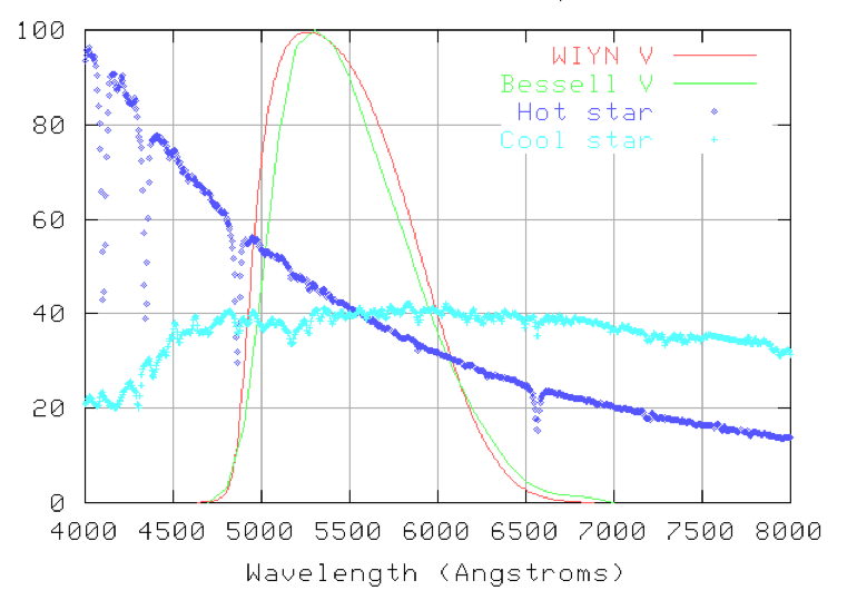
often in the profile of the filter. Figure 24 shows two V
filters used at the Kitt Peak National Observatory in Arizona. The WIYN V filter has a
sharper increase in transmission on the blue side of the profile than the Bessell V
filter, allowing more light to enter from hot, blue stars than from cool, red stars. This
creates a systematic error that makes blue stars seem a bit brighter than red stars when
observed through the WIYN V filter.
Figure 24: plot by Michael Richmond showing two different V filters and the spectra of hot and cold stars, demonstrating why correcting for colour terms is necessary when performing high-accuracy photometry (see text for details).
Fortunately, it is straightforward to correct for this systematic error by observing a field with
many standard stars possessing a range of colours. The advantage of observing a single field is
that all of the stars will then be at the same airmass and hence extinction effects are
cancelled out. If this is not possible, you can use many observations of standard stars in
different fields. We have already seen that:
\[m_{\rm zp} = m_{\rm std} - m_{ {\rm std},0,i}.\]
Hence, if the telescope, instrument, filter and detector combination being used matches that of
the photometric system perfectly, we can write:
\[m_{\rm std} - m_{ {\rm std},0,i} - m_{\rm zp} = 0.\]
In practice, however, the observer's equipment is never identical to that used to define the
photometric system, resulting in the above equation being modified to:
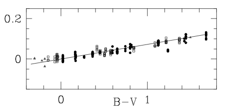
\[m_{\rm std} - m_{ {\rm std},0,i} - m_{\rm zp} = c C,\]
where \(c\) is the colour term, and \(C\) is the colour index (e.g \(B-V\)). Hence, the colour
term is equal to the gradient in a plot of \(m_{\rm std} - m_{ {\rm std},0,i} - m_{\rm zp}\)
against \(C\), i.e a plot of the difference between the catalogue magnitudes of the standard
stars and their calibrated magnitudes as a function of colour; the \(y\) intercept is set to
zero by using a zero point calculated from a star of \(B - V = 0\). An example of such a plot is
shown in figure 25, which has a gradient of 0.072. You can see from this
plot that use of colour terms are necessary to obtain accuracies of order 0.01 magnitudes (i.e
1% in flux). If your requirements are less accurate, you can ignore colour terms, as we will do
for the remainder of this course.
Figure 25: a plot of the difference between the catalogue magnitudes of a set of standard stars and their calibrated magnitudes (y axis) as a function of colour (x axis). The gradient of the line is equal to the colour term.