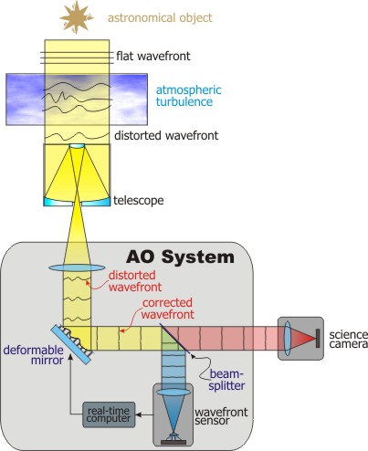
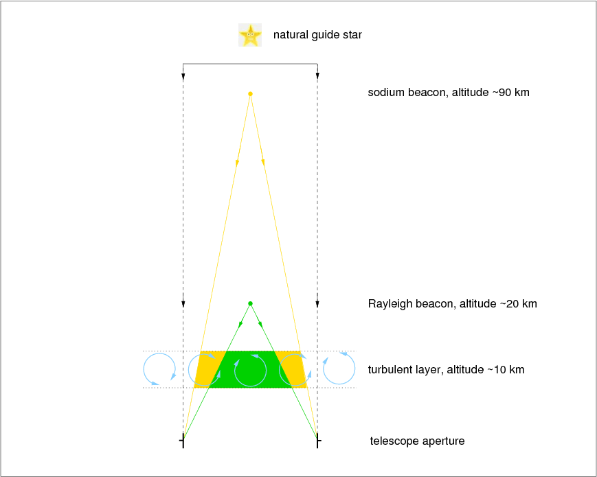
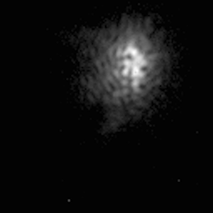
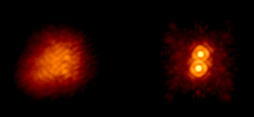
In the first lecture, we saw how the seeing was the dominant factor controlling image quality for telescopes of moderate size and larger. Whilst active optics counteracts the effect of gravity and other deformations on the telescope mirrors, adaptive optics is a way of correcting for seeing, and taking advantage of the potential for improved resolution offered by large telescopes. Before we discuss how adaptive optics works, I will introduce three terms which quantify the effects of turbulence in the Earth's atmosphere on a wavefront propagating through it.

Fried parameter

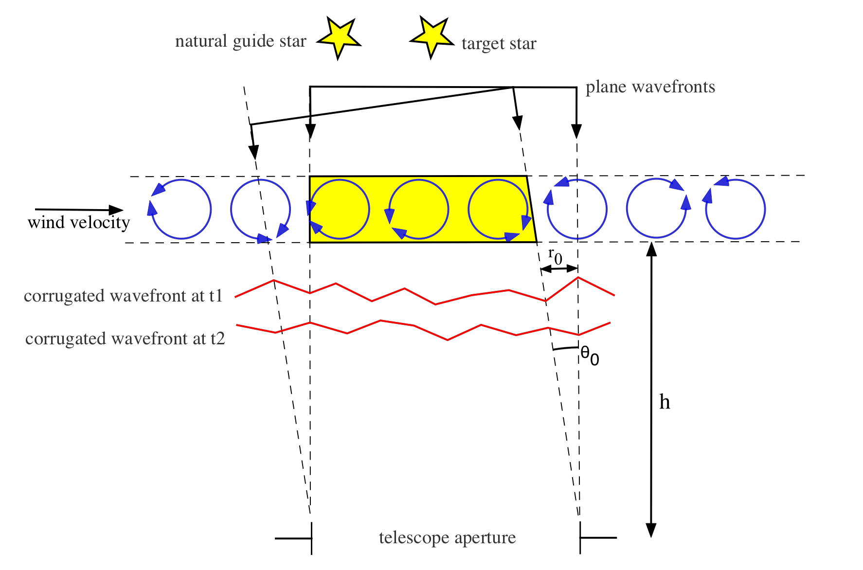
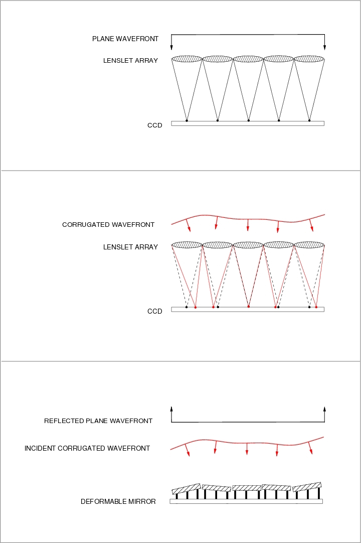
As we showed in figure 6, turbulence in the atmosphere randomly distorts the plane wavefronts from distant stars. Over a short distance, the corrugated wavefront can be considered approximately planar. The Fried parameter, \(r_0\) - pronounced free-d - indicates the length over which the wavefront can be considered planar. This is shown schematically in figure 61. As we can see from this figure, the Fried parameter is also approximately equal to the size of the turbulent cells themselves.

The larger the Fried parameter, the better the atmospheric conditions. At a good observing site, the Fried parameter has a typical value of \(r_0 = 10\) cm, at an optical wavelength of \(\lambda = 500\) nm. Theoretically, the Fried parameter is predicted to vary with wavelength as \(r_0 \propto \lambda^{6/5}\). Accordingly, the Fried parameter at near-infrared wavelengths (\(\lambda = 2.5 \mu\)m) should be \(r_0 \sim 70\) cm. This expectation is borne out by observations

Coherence Time

In figure 61, two wavefronts are shown at times \(t_1\) and \(t_2\). The turbulent cells responsible for distorting the wavefront generally evolve on long timescales. The reason the wavefront changes between time \(t_1\) and time \(t_2\) is because the wind moves the turbulent cells across the sky. A measure of the timescale on which the wavefronts change is the time taken for a turbulent cell to move it's own size; the so-called coherence time. The coherence time is given by \[t_0 = t_2 - t_2 = \frac{r_0}{v},\] where \(v\) is the wind speed. At a good observing site on a typical night, \(v = 10\) m/s and \(r_0 = 10\) cm at \(\lambda = 500\) nm. Hence \(t_0 \sim 10\) ms. In the near-infrared, the coherence time is longer (because the Fried parameter is larger). The coherence time in the near-infrared is nearer 70 ms. Any adaptive optics system which aims to correct for seeing, must change it's correction at the coherence timescale. Thus, an adaptive optics system in the near-infrared can operate more slowly than in the optical.

Isoplanatic angle

Consider the two stars in figure 61. They are sufficiently close that the light from them passes through roughly the same turbulent region (shaded in yellow in the figure). The isoplanatic angle is the angle two stars can be separated, and still have their light pass through the same turbulent region. The estimate shown in figure 56 is that the two beams are separated by the size of one cell \(r_0\) at the height of the turbulent layer \(h\). It follows that the isoplanatic angle is given by \[\theta_0 = r_0 / h.\] Once again, at a good observing site on a typical night, \(v = 10\) m/s and \(r_0 = 10\) cm at \(\lambda = 500\) nm. Hence \(\theta_0 \sim 10^{-5}\) radians, which is 2". Once again, the isoplanatic angle in the near-infrared is much larger (around 14"). The isoplanatic angle determines the area on the sky over which adaptive optics correction is effective. This implies that much wider fields (and hence more extended objects) can be corrected with adaptive optics in the infrared than in the optical, making the technique much more attractive in the infrared. The increased isoplanatic angle in the infrared also means that many more natural guide stars are available, as discussed below.

Principles of adaptive optics

The principles of adaptive optics correction are shown in figure 62. A plane wavefront from a star is corrugated by turbulence in the Earth's atmosphere. The diverging beam beyond the focal plane of the telescope is then made parallel using a collimator, and the collimated beam reflects off a deformable mirror, which is adjusted in shape to match that of the wavefront. As a result, the reflected wavefront becomes planar again, and the corrected beam is then focused and detected by a science camera. The shape of the deformable mirror is adjusted hundreds of times a second, using information provided by a wavefront sensor, which picks off the (unwanted) blue light in the beam using a dichroic beamsplitter. Note that the shape of the wavefront is independent of wavelength, which is why it is then possible to sense and correct at different wavelengths

Wavefront Sensors

The key to adaptive optics is being able to measure the shape of the wavefront, so the deformable mirror can correct for it. There are many different designs of wavefront sensor, but the simplest to understand is the Shack-Hartmann sensor, which is described here. The principles of the Shack-Hartmann sensor are shown in figure 63. The Shack-Hartmann wavefront sensor consists of a lenslet array which the corrugated wavefront is incident upon. A plane wavefront incident on the lenslet array would produce a regular series of spots on a high-speed detector in the focal plane - the positions of these spots can be considered reference positions. A corrugated wavefront, on the other hand, would produce irregularly spaced spots, where the tilt of each section of the wavefront can be determined by measuring the displacement of the spot from the reference positions (measured by illuminating the lenslet array with a plane wavefront).

The tilt of the wavefront at each lenslet is then used to set the tilt of each corresponding element in the segmented deformable mirror (to a value equal to half of the tilt of the wavefront), so that the reflected wavefront becomes planar. For accurate correction, it is essential that the delay between sensing the wavefront and adjusting the shape of the deformable mirror is no greater than the coherence time of the atmosphere, which is typically a few milliseconds in the optical part of the spectrum at a good astronomical site. Hence high-speed computer processors to measure the wavefront and move the mirror in a real-time correction loop are also an essential component of any adaptive optics system. It is also vital that the sizes of the lenslets, and hence the mirror segments, are well matched to the typical values of the Fried parameter at the observing site and wavelength of interest.

These practical considerations mean that adaptive optics systems in the near-infrared can have fewer elements, be larger and operate more slowly than in the optical. As we saw when we discussed the isoplanatic angle, they can also correct larger areas of sky. For these reasons, AO is much easier to implement in the infrared than the optical.

Laser Guide Stars

In order for a Shack-Hartmann wavefront sensor to measure the tilts of a wavefront accurately, it is necessary to observe a bright point source to provide a sufficient signal-to-noise ratio in the short exposure times. It is possible that the science target itself can be used to sense the wavefront, e.g. if it has a bright, point-like central structure, such as an active galactic nucleus or young stellar object. Unfortunately, many astronomical targets are either faint, extended, or both. One way round this is to observe a bright star close to the target, but such a natural guide star would have to be within the isoplanatic angle of the target, otherwise the target and guide stars would be sampling different turbulence in the atmosphere (as shown in figure 61). In the near-infrared the isoplanatic angle is 10-20", so only a very small number of stars can be observed using natural guide stars. The only way of significantly increasing the sky coverage is to generate an artificial guide star close to the target using a laser: a so-called laser guide star. A schematic of a laser guide star is shown in figure 65, whilst a photograph of a laser guide star in operation on the VLT in Chile is shown on this course's homepage.

There are two types of laser guide star. The first, known as a Rayleigh beacon, uses the Rayleigh back-scattering of light from molecules in the lower atmosphere to produce an artificial star at altitudes of approximately 20 km. The second type is the sodium beacon, which uses a laser tuned to the yellow sodium D lines around 589 nm. This excites sodium atoms (deposited by micrometeorites) in the mesosphere at an altitude of approximately 90 km, which subsequently re-emit the light, producing an artificial star, as shown in figure 65.

Although much more more costly and complex than Rayleigh beacons, sodium beacons have one major advantage: they do not suffer as badly from the cone effect, resulting in superior adaptive optics correction. This is shown schematically in the bottom panel of figure 65, where it can be seen that the higher altitude of the sodium beacon means that it shares much more of the turbulence experienced by light from the star than the lower-altitude Rayleigh beacon.

No matter which type of laser beacon is used, an artificial star is created well above the typical altitudes at which turbulence occurs. The artificial star can be placed within the isoplanatic angle of the science target, resulting in 100% sky coverage for adaptive optics. Since the laser light is monochromatic, a simple notch filter can be used to direct all of the laser light to the wavefront sensor, leaving the rest of the light to be directed to the science detector.

Performance of adaptive optics

We have already seen that the spatial resolution of a seeing-limited image is usually characterised by the full-width at half-maximum (FWHM) of a stellar profile, measured in arcseconds. This method becomes unreliable, however, as the spatial resolution approaches the diffraction limit, as measurement of the FWHM becomes complicated by the presence of diffraction rings. A more useful measure in this case is the Strehl ratio, which is the ratio of the intensity at the peak of the observed seeing disc divided by the intensity at the peak of the theoretical Airy disc, as shown in figure 66.

Most large telescopes in the world are now equipped with adaptive optics systems. The most advanced such systems incorporate laser beacons and wavefront sensors/deformable mirrors with 1000+ elements, delivering diffraction-limited imaging in the infrared across most of the sky. However, diffraction-limited imaging on large-aperture telescopes is still not achievable in the optical. As discussed above, this is due to the lower values of the Fried parameter and coherence time, implying that an unfeasibly large number of adaptive elements and corrections per second would be required.

Figure 67, below, shows some examples of adaptive optics in action.