Obtaining spectroscopic data on astronomical objects is at the heart of observational astronomy. Photometry through different coloured filters can provide crude information on the spectrum of an object, but what if we need finer detail? Perhaps we wish to study the absorption lines present in a star's spectrum, or measure a star's radial velocity through the shift in those lines. The astronomical spectrograph is designed for this purpose. An astronomical spectrograph splits, or disperses, the light from a source into its component wavelengths. Some means of dispersing the light is therefore required. This function used to be performed by a prism, which exploits the fact that light of different wavelengths are refracted by different amounts, with blue light being refracted more than red light. However, prisms are inefficient, as light is lost at each air-glass surface (see figure 87). In addition, the amount of dispersion is not very high, and not easy to control.
L15: Spectrographs I design principles
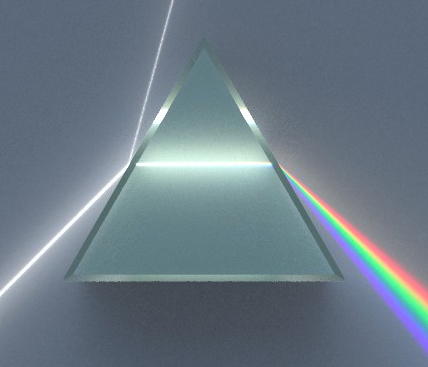
Figure 87: Dispersion of light by a prism. Note the loss of light at each air-glass surface, which makes prisms inefficient.
Gratings
The almost universal choice for the dispersing element in modern astronomical spectrographs is the diffraction grating. There are two types of diffraction grating in use:
- a transmission grating, where a large number of fine, equidistant, parallel lines are ruled onto a transparent glass plate so that light can pass between the lines, but not through them.
- a refection grating, where the lines are ruled onto a reflective piece of glass so that only the light between the lines is reflected.
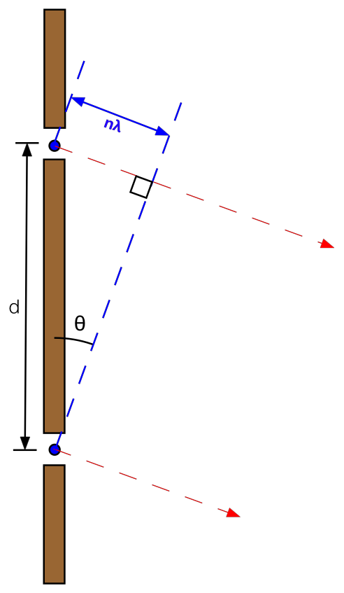
In figure 88, I show a simplified diffraction grating, where we have two gaps between the ruled lines acting as secondary sources. The path length between these two sources to a distant detector is given by \(d\phi = d\sin\theta\). When this path length is equal to an integer number of wavelengths, we will get constructive interference. Hence, the condition for constructive interference is written as \[n\lambda = d\sin\theta.\] This equation is known as the grating equation, and is fundamental to understanding how gratings work.
If we imagine monochromatic light falling on our grating, we will get constructive interference, and thus beams of light, where \(n=0,1,2,...\), and so on. These are referred to as the zeroth, first and second orders. Now consider what happens when white light is incident on our grating. In the zeroth order, \(n=0\) and the angle at which constructive interference occurs, \(\theta\), is independent of wavelength. The zeroth order is not dispersed. In the first orders \(n = \pm 1\), the grating equation implies that \(\theta\) must increase as \(\lambda\) increases. Thus, the angle at which constructive inteference occurs is wavelength dependent, and dispersion occurs. This is shown in figure 89.
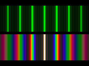
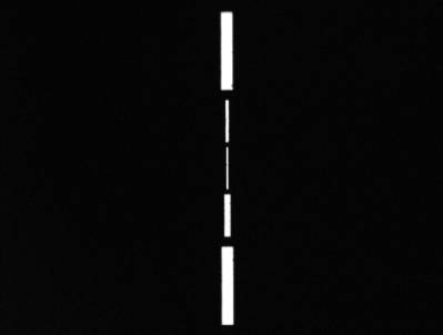
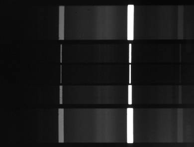
Figure 89: Photograph showing the diffraction pattern produced by a monochromatic light source (top) and a white light source (bottom) incident on a diffraction grating. The central bright line is the zeroth order, with orders ±1, ±2 and ±3 shown either side of this. Notice the larger dispersion in the higher orders, as predicted by the grating equation. We will discuss the origin of the fainter lines between the bright lines in the next lecture.
Basic spectrograph design
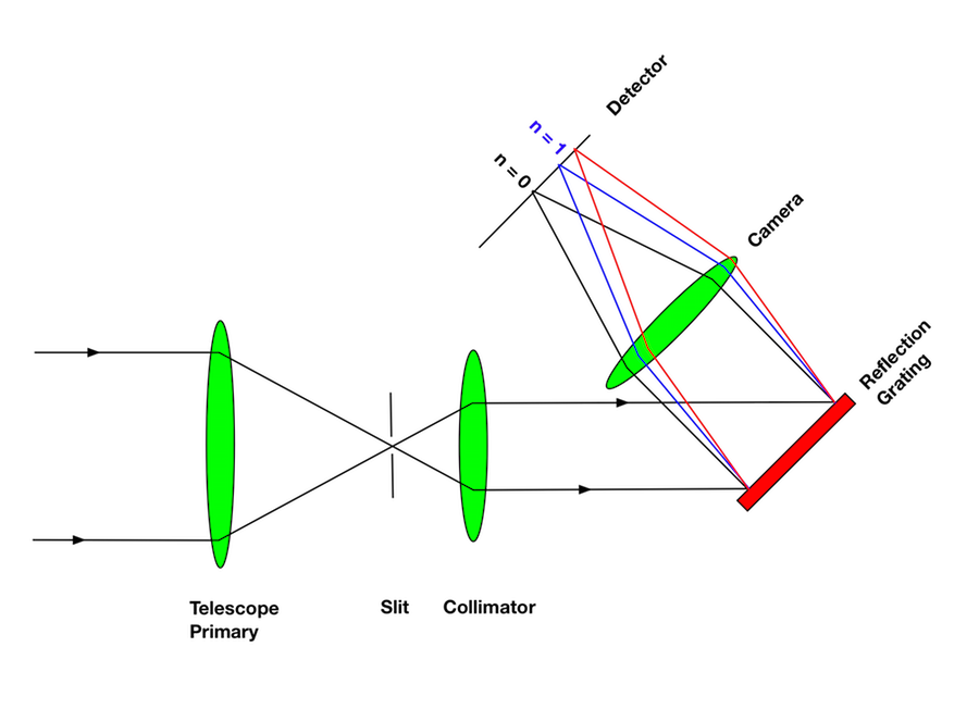
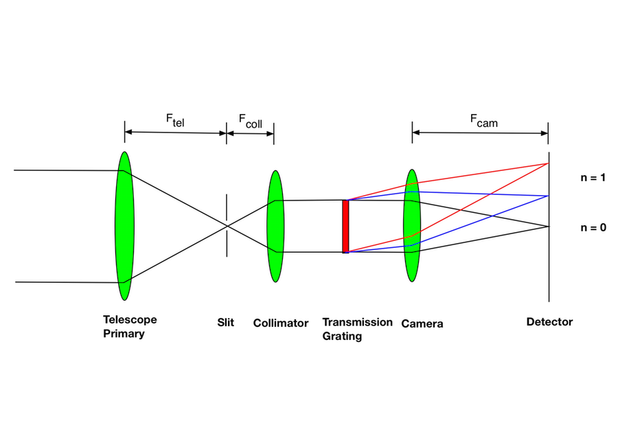
Most spectrographs use the same design, based on the re-imager we saw in the previous lecture. Schematics of spectrographs, using transmission and reflection gratings, are shown in figure 90. The five basic components of an astronomical spectrograph are the slit, collimator, grating, camera and detector. The roles of each of these components are described in more detail below.
Slit
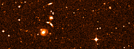
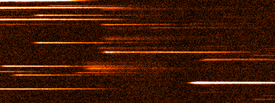
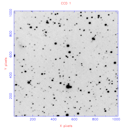
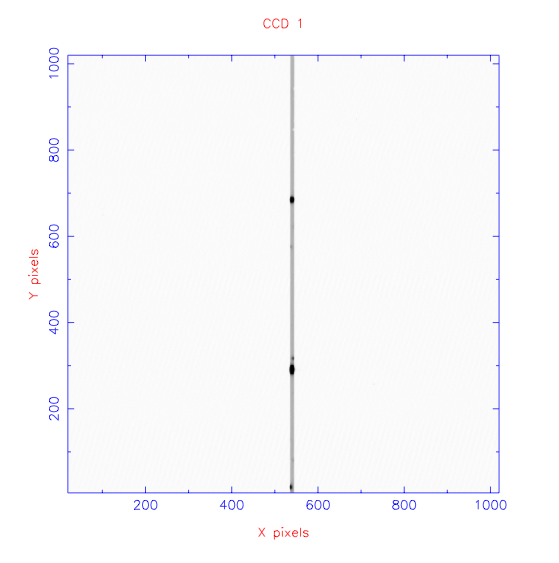
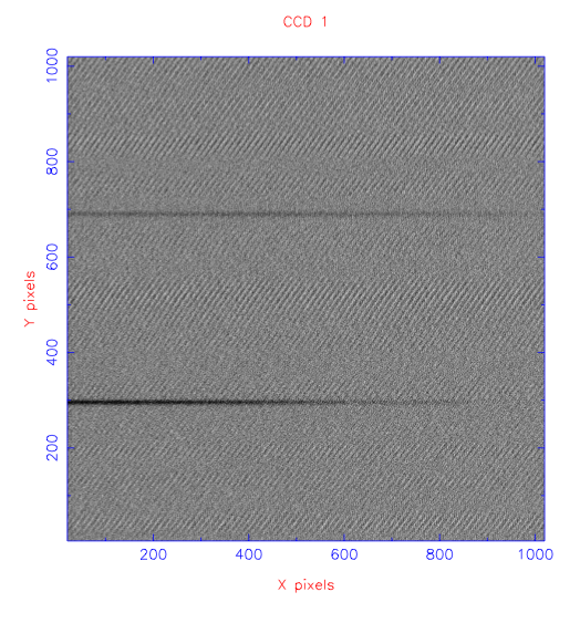
The slit is a mask with a narrow rectangular aperture that is placed in the focal plane of the telescope. The slit has two main functions. First, the slit acts as a means of isolating the region of interest on the sky. Without a slit present, the spectra from sources either side of the target would overlap figure 91, contaminating the target spectrum. Additional sky background from either side of the target would also be recorded, degrading the signal-to-noise ratio of the spectrum. By putting a slit in the focal plane of the telescope, only light falling on the slit may enter the spectrograph, as shown in figure 92.
The second function of the slit is to provide stable spectral resolution. This can be understood by noting that a spectrum is essentially an infinite number of images of the telescope focal plane, each shifted slightly in wavelength. Hence, without a slit present, the spectral resolution of an object would be defined by the width of the object. For a point source like a star the would be defined by the seeing. However, since seeing varies with time, the spectral resolution would then vary with time. The solution is to illuminate a narrow slit with the source, so that the spectrum becomes an infinite number of images of the slit, not the source. The minimum width of any spectral lines would then be defined by the slit width, and would hence be stable.
Spectrographs re-image, or project, the slit in the focal plane of the telescope onto the detector, which lies in the focal plane of the camera. As we discovered when looking at re-imagers, the ratio of the camera to collimator focal lengths determines the magnification of the image of the slit on the detector: \(M = F_{\rm cam} / F_{\rm coll}\). Hence a slit of width 50 μm in a spectrograph with a collimator of focal length 500 mm and camera of focal length 250 mm would be projected to a width of 25 μm on the detector. We will see what sets the optimal slit width, when we discuss spectral resolution in the next lecture.
Collimator
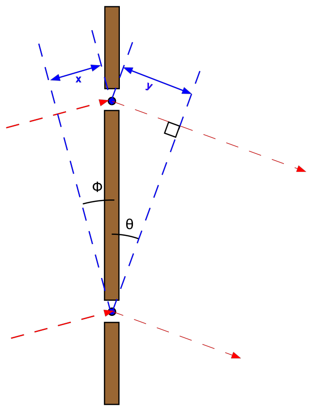
When we derived the grating equation, we assumed the light was arriving perpendicular to the grating. In general the light will arrive at the grating at an angle \(\phi\), and this will add an additional phase shift to the light emerging from each gap between the grating lines. The situation is shown in figure 95.
In figure 95, we see that the new phase shift between the two sources is \(x + y\). Since \(x = d\sin\phi\) and \(y = d\sin\theta\), a modified version of the grating equation to account for this is \[n\lambda = d (\sin\theta + \sin\phi).\] Without a collimator, the diverging light from the slit would hit the grating, resulting in variable angles of incidence as a function of position on the grating. From the equation above, we see that varying the angle of incidence, \(\phi\), results in changes to the angle of diffraction, \(\theta\). Hence the same wavelength of light in the same order would be imaged onto different positions on the detector, blurring the resulting spectrum. With a collimator, however all angles of incidence on the grating are equal and no such blurring would result.
Grating
As discussed above, the grating splits the light into its component wavelengths. The modified grating equation above shows that by varying \(\phi\), the wavelength that gets diffracted into angle \(\theta\) can be varied. This will affect the location on the detector of each wavelength. Hence most spectrographs have gratings that can be tilted in order to adjust the start and end wavelengths of the spectrum.
Camera
The role of the camera in an astronomical spectrograph is to collect the spectrally-dispersed beams from the grating, which are still collimated, and make them converge so that the spectrum is imaged onto the detector. The camera can be either a lens, mirror, or catadioptric system.
Detector
The dispersed light is ultimately imaged by the spectrograph onto the detector, forming a spectrum, as shown in the bottom-right panel of figure 92. We can define the direction along the slit (i.e. the vertical direction in the right panel of figure 92) as the spatial axis, and the direction along the spectrum (i.e. the horizontal direction in the right panel of figure 92) as the dispersion axis.