In the previous lecture we saw the basics of spectrograph design, and used an idealised grating with only two lines to derive the grating equation. However, astronomical gratings can have many thousands of lines ruled onto their surface. Why? In addition, the gaps between the lines (which act as secondary sources) have a finite thickness. How does this affect the diffraction pattern produced by the grating?
L16: Spectrographs II detailed design
Realistic Gratings
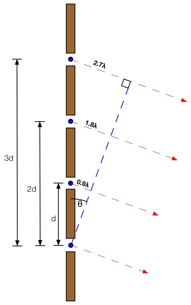
We shall ignore for a moment the effect of the finite size of the gaps, and look at the effect of multiple lines. Figure 96 shows a multi-lined grating, with 4 gaps between the ruled lines acting as secondary sources. I have chosen \(\theta\) such that the bottom two gaps have a path difference \(d\sin\theta\) which is almost equal to a whole number of wavelengths. If these were the only two gaps we would almost have constructive interference, and the diffraction pattern in this direction would be quite bright.
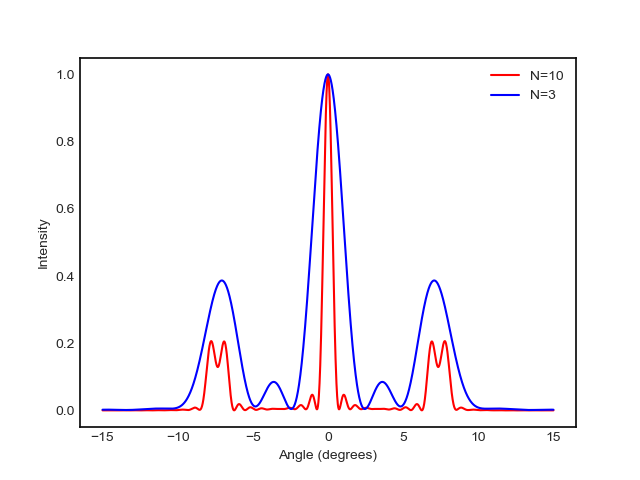
However, the path difference between the first gap and successive gaps is larger. This means that we are adding light that is increasingly out of phase. From the diagram we see the \(N^{\rm th}\) gap would have a path difference of \(Nd\sin\theta\). For large enough \(N\) this will destructively interfere with the light from the first gap, reducing the brightness of the diffraction pattern. The effect of multiple slits is therefore to make the diffraction pattern drop off more rapidly away from the peaks. The rate at which the diffraction pattern drops off in intensity increases with a larger number of lines. This is shown in figure 97.
Another effect of multiple lines is also shown in figure 96. Notice that when the phase difference between the first two slits is \(\lambda\), the phase difference between slits one and three is \(2\lambda\) and so on. Thus in direction we still have constructive interference. Adding mutliple slits has not changed the position of the maxima, and they still obey the grating equation.
However, away from the main peaks, we will get smaller sub-peaks, where pairs of gaps (say, gap 2 and gap 4) constructively interfere. These smaller peaks are shown in figure 97.
What about the finite width of the gaps? Figure 97 shows the familiar diffraction pattern you would get from a single gap of finite width. The effect of many gaps of finite width is to multiply the idealised (narrow gaps) patterns by the diffraction pattern of a single gap. This makes the zeroth order the brightest by far. In figure 86 I have used relatively narrow gaps, so the diffraction pattern of a single gap is quite wide. In real spectrographs the gaps are wider than this, and the zeroth order is much brighter than the first and second orders. This is a problem that must be addressed, as the zeroth order is undispersed and not useful for spectroscopy! By ruling the lines at an angle to the surface of the grating - known as a blaze - we can direct light into the order of interest. For the curious, this is explained in more detail in Vik Dhillon's old notes.
Now we understand the effect the grating properties have on the diffraction pattern, we look at some of the details of spectrograph design.
Spectral Range and Order Overlap
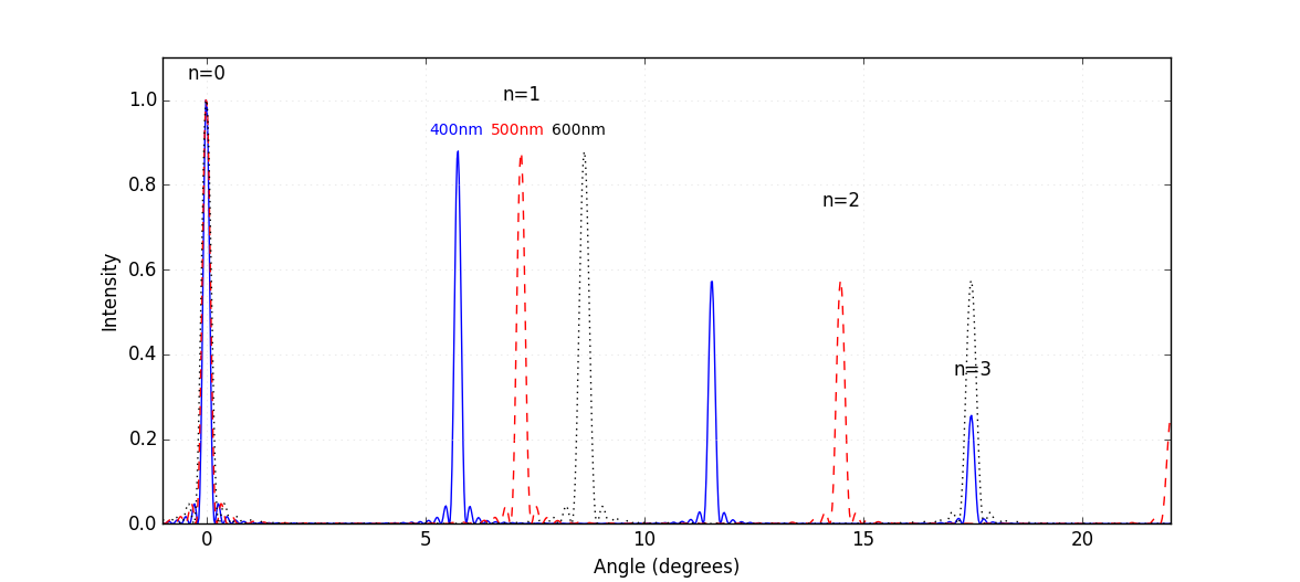
A big problem for spectrographs is that the various orders overlap. This is shown in figure 98, and can be understood from the grating equation, \(n\lambda = d\sin\theta\). At any given angle \(\theta\) the light could have wavelength \(\lambda/n\) for \(n=1,2,3...\). The way round this is to insert order sorting filters into the collimated beam, which only allow a restricted wavelength range to pass, avoiding overlap. However, this obviously restricts the range of the spectrograph. The best case is in the first order, where for a given wavelength \(\lambda\), a spectral range of order \(\lambda\) is observable without overlap.
Dispersion
In a given order, what is the relationship between wavelength \(\lambda\) and angle \(\theta\)? We can use the grating equation \(n\lambda = d\sin\theta\) to show \[\frac{d\theta}{d\lambda} = \frac{n}{d \cos\theta}.\] This is known as the angular dispersion (measured in, say, radians per Angstrom) and it is greater for small line spacings, \(d\). It also increases with spectral order \(n\). It is usually more convenient to talk about the linear dispersion - the rate at which \(\lambda\) changes with distance along the detector \(x\). If the spectrograph camera has a focal length \(F_{\rm cam}\), then an angle \(\theta\) corresponds to a position \(x = F_{\rm cam} \theta\). Therefore \[ \frac{dx}{d\lambda} = \frac{dx}{d\theta} \frac{d\theta}{d\lambda} = \frac{nF_{\rm cam}}{d\cos\theta}.\] The diffraction angle \(\theta\) is usually quite small, so we can write \( dx/d\lambda \approx nF_{\rm cam}/d\). The linear dispersion thus increases with the focal length of the camera, the spectral order, and increases with smaller line spacings.
The equation above is often inverted to give the reciprocal linear dispersion, i.e. the wavelength range for a particular length at the detector.
What kind of line spacings are practical? For a given size of chip, \(\Delta x\), the range of wavelengths covered will be given by \(\Delta\lambda\), where \[\frac{\Delta \lambda}{\Delta x} = \frac{d}{nF_{\rm cam}}.\] There is no point in this spectral range being larger than the amount which would cause order overlap. If we are working in the first order, \(n=1\), this is of order \(\lambda\). So we have \(\Delta \lambda \approx d \Delta x/F_{\rm cam} \sim \lambda \), which we can re-write to get a lower limit on the line spacing as \[\frac{d}{\lambda} \sim F_{\rm cam} \Delta x.\] A typical CCD has a size of roughly 3 cm. A reasonable choice for line spacing would be \(d/\lambda \sim 10\) - this would imply a camera of focal length 30 cm. Wider spaced rulings with \(d/\lambda \sim 100\) would need a camera of focal length 3 m, which would be as big as a moderately large telescope!
At optical wavelengths of \(\lambda = 500\) nm, \(d/\lambda \sim 10\) implies \(d = 5\mu\)m. This is often expressed in the number of lines per mm - in this case 200 lines/mm. For a reasonable sized camera and observing in the first order, this would give a spectral range roughly the same as the limit imposed by order overlap. We could use smaller line spacings to increase the dispersion at the expense of spectral range - such gratings might have 1,000 lines/mm. To see why we would do this, we need to look at what sets the spectral resolution of a spectrograph.
Spectral Resolution
The concept of spectral resolution is closely linked to spatial resolution, which we discussed in the first lecture. Diffraction gratings with more lines produce sharper diffraction patterns, allowing us to resolve two neighbouring wavelengths. This is shown schematically in figure 99. We can apply the same Rayleigh Criterion we adopted for imaging and say that two wavelengths are resolved when the peak of one diffraction pattern lies on top of the minimum of the other. To find the resolution of a spectrograph we thus need to find the distance to the first minimum.
It is possible to show that the diffraction pattern produced by a grating with \(N\) lines, each of width \(a\) and with spacing \(d\) is given by \[I = I_0 \left(\frac{\sin\alpha}{\alpha}\right)^2 \left( \frac{\sin N\beta}{\sin \beta} \right)^2,\] where \(\alpha = (\pi a / \lambda) \sin\theta\) and \(\beta = (\pi d / \lambda) \sin\theta\).
The zeros of this pattern are given when \(\sin N\beta = 0\), which can be manipulated to show \[\sin\theta_{\rm zeroes} = \frac{n'\lambda}{Nd},\] where \(n'\) is an integer that labels the zeros, i.e \(n' = 1,2,3...\). To get the angular distance from one zero to the next we note that \(\Delta \theta = \Delta n' \frac{d\theta}{dn'}\), and \(\Delta n' = 1\) - which gives \(\Delta \theta = \lambda/Nd\cos\theta\). Since \(\theta\) is small we can use \(\cos\theta \approx 1 \) to give \[\Delta\theta \sim \frac{\lambda}{Nd}.\] This is the angle between one zero to the next, and it depends on the wavelength, the number of lines and the line spacing. However, we really want to know what wavelength range this angle corresponds to. For that we can use \(\Delta\lambda = \Delta \theta \frac{d\lambda}{d\theta}\). We showed above, using the grating equation, that \(\frac{d\lambda}{d\theta} = d\cos\theta / n \approx d/n\). Therefore, we have \[\Delta \lambda = \lambda / Nn.\] This is usually expressed as the resolving power of a spectrograph \(R = \lambda / \Delta \lambda = Nn\). The resolving power can be increased by working in a higher order, or by increasing the total number of lines in the grating, \(N\). For a fixed-size grating, this means increasing the number of lines/mm.
The resolution discussed above is the limit imposed by diffraction. However, just as in imaging, other factors mean that the diffraction limited resolution may not be reached. The spectral resolution of a spectrograph is usually limited by the slit width, or the physical size of the pixels in the CCD, as described below.
Slit Width
The diffraction patterns shown above are the result of the light from a point source falling on the grating. However, we have seen that it is useful to think of a spectrum as essentially an infinite number of images of the slit, each shifted slightly in wavelength. If the projected slit width at the detector is much less than the limiting resolution of the spectrograph, then no loss of resolution will result. However, if the slit is widened so that the width of its image in the spectrum rises above the limiting resolution, then it is the width of the slit that will define the resolution of the spectrum, not diffraction.
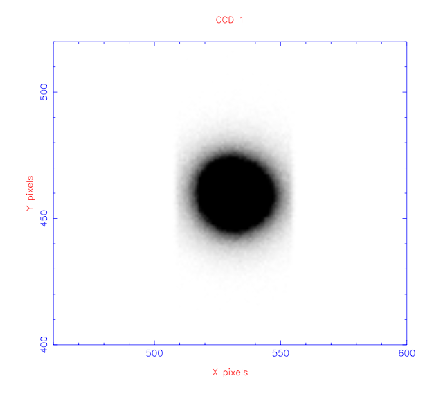
To maximise spectral resolution, therefore, it seems obvious that the slit width should always be kept smaller than the limiting resolution. Unfortunately, this is rarely possible, as the slit would be so narrow compared to the seeing disc of the star that very little light would pass into the spectrograph. This trade-off between spectral resolution and throughput is illustrated in figure 100, which shows images of the same star passing through a wide slit and a narrow slit. In the wide slit case, all of the light is able to pass into the spectrograph, but the resolution would be defined by the seeing (and image motion due to guiding errors), not the slit. In the narrow slit case, the resolution of the spectrograph would be defined by the width of the slit and would more closely approach the limiting resolution, but only a fraction of the light from the star would pass through the slit.
detector pixel size
The size of the pixels in the CCD detector also has an influence on the effective resolution of a spectrograph. Specifically, if our pixels are larger than a resolution element, the resolution will be set by the size of our pixels. As with imaging, we usually try to have at least two pixels per resolution element for optimal sampling. Since in practice it is the slit width that usually defines the spectral resolution, spectrographs are usually designed so that the slit is matched in width to the seeing, and projects to two pixels on the detector. All of this can be quite confusing, and it is a common mistake to mix up spectral resolution and dispersion. The best way of clarifying this is to go through a worked example.
Spectral resolution and velocities
As a rough guide, spectrographs with \(R < 1000\) are regarded as low resolution and they generally do not allow the spectral lines from astronomical sources to be resolved. Spectrographs with \(1000 < R < 10,000\) are regarded as intermediate resolution, and these do enable the study of the broadest spectral lines. However, only high-resolution spectrographs, with \(R> 10,000\), enable the narrow spectral lines emitted by most stars to be studied in detail. Note that, in comparison, broad-band photometry has an effective spectral resolution of \(R \sim 5\).
One use of spectra is to measure the Doppler shifts of spectral lines. The smallest shift that can be detected is set by the spectral resolution. Since the Doppler shift is given by \(\Delta\lambda / \lambda = \Delta v/c\), and the resolving power \(R = \lambda / \Delta \lambda\), it follows that the smallest velocity shift that can be measured by a spectrograph is roughly \[\Delta v = c/R.\] For intermediate resolution spectrographs with \(R\sim 3000\), this corresponds to velocities of order 100 km/s. To detect the tiny Doppler wobbles induced by exoplanets, which are of order metres per second, requires very high spectral resolution.
Spectrograph Design - A worked example
-
A grating of width 50 mm and 300 lines/mm is used to create a second order spectrum. What is the limiting spectral resolution at 500 nm?
The diffraction limit to resolution is \(\Delta \lambda = \lambda / Nn\). In this case \(n=2\) and \(N = 50 \times 300 = 15000\) lines. Therefore \[\Delta \lambda = \frac{550 \times 10^{-9}}{2 \times 15000} = 1.8 \times 10^{-11} {\rm m} = 0.18 \unicode{xC5}.\]
-
If the spectrograph has a camera of focal length 300 mm, what is the reciprocal linear dispersion in \( \unicode{xC5}\)/mm?
The reciprocal linear dispersion is given by the inverse of the linear dispersion \[\frac{d\lambda}{dx} = d\cos\theta / n F_{\rm cam} \approx d/nF_{\rm cam}.\] Since the grating has 300 lines/mm the line spacing is 3 \(\mu\)m. Remembering that \(n=2\), we have \[\frac{d\lambda}{dx} = \frac{3\times 10^{-6}}{2 \times 300 \times 10^{-3}} = 5\times10^{-6}.\] Units get a bit confusing here. The above reciprocal dispersion is in meters per meter. We want to convert it to \(\unicode{xC5}\) per mm, so we multiply by \(10^7\) to get \[\frac{d\lambda}{dx} = 50 \, \unicode{xC5} \, {\rm mm}^{-1}.\]
-
If the detector has 15 \(\mu\)m pixels, will we achieve the diffraction limited resolution?
Each pixel is \(15\times 10^{-3}\) mm. With a reciprocal linear dispersion of \(50 \,\unicode{xC5} \, {\rm mm}^{-1}\), one pixel corresponds to \[d\lambda = 50 \times 15\times 10^{-3} = 0.75 \unicode{xC5}. \] This is more than the diffraction limited resolution of 0.18 \(\unicode{xC5}\), so we will not reach this limit.
-
How might we change the spectrograph to reach the diffraction limit?
It isn't feasible to make CCDs with much smaller pixels. Therefore we need to reduce the reciprocal linear dispersion to 12 \(\unicode{xC5} \, {\rm mm}^{-1}\). Changing the line spacing \(d\) will also affect the diffraction limited resolution. We have to increase the camera focal length.
To reach a reciprocal linear dispersion of 12 \(\unicode{xC5} \, {\rm mm}^{-1}\) requires a focal length of 12,500 mm, or 1.25 m! This is similar in size to many telescopes, and illustrates why reaching the diffraction limit is not normally practical.
-
Suppose we leave the spectrograph unchanged. I want to use the spectrograph on a 2m \(f/10\) telescope, where the seeing is 1 arc second. What physical size must the slit be, and what collimator focal length should I use?
If the typical seeing is 1", then it would be best to use a slit width of approximately this size so as to obtain reasonable throughput whilst still ensuring that the resolution of the spectrograph is defined by the slit.
For optimal sampling, the 1" slit should project to at least 2 pixels on the detector. The platescale of the telescope is 206265 / 20000 = 10.3 "/mm, so the physical width of the slit is approximately 100 μm, which must project to 2 x 15 = 30 μm. Hence the magnification of the spectrograph must be 0.3, implying that the ratio of camera to collimator focal lengths must also be 0.3. Thus, the collimator focal length must be 900 mm.
-
OK. So what's the resolving power of my spectrograph if I'm observing at 550 nm?
The spectral resolution is set by the slit width. The slit projects to 2 pixels, or 30 μm. Since the reciprocal linear dispersion is \(50 \,\unicode{xC5} \, {\rm mm}^{-1}\), the resolution is \[\Delta \lambda = 50 \times 30 \times 10^{-3} = 1.5 \unicode{xC5}\]. The resolving power is \(R = \lambda / \Delta \lambda = 550 \times 10^{-9} / 1.5 \times 10^{-10} \approx 3600\). This is a medium resolution spectrograph.
-
Suppose I can get my hands on a grating of the same size, but with 600 lines/mm. If I leave everything else unchanged, what will my spectral resolution be?
With the same re-imaging lenses, the slit will still project to two pixels, or 30 μm. However, the reciprocal linear dispersion will halve. The resolution will therefore double - to \(R = 7200\).
-
If my detector has 2048 pixels in the spectral direction, what's my spectral range?
With a new reciprocal dispersion of \(25 \,\unicode{xC5} \, {\rm mm}^{-1}\) and 2048 pixels of 15 μm, the spectral range is \[15 \times 10^{-3} \times 2048 \times 25 = 768 \unicode{xC5} = 77 {\rm nm}.\]